ACMC - Class weighting and MCC | Agneev’s DS/ML lab book

Categories:

Machine Learning Computer Vision Python Metric

Tags:

TensorFlow 2, Keras, Matplotlib, Seaborn, Pandas, Scikit-learn, Matthews correlation coefficient

Hello! In the previous post, we looked at the pros and cons of using undersampling for dealing with the imbalance inherent in the Archie Comics Multiclass (ACMC) dataset. The next thing to explore, logically, would be the opposite tactic - oversampling to increase the number of samples in the minority classes. That’s not what we are going to do today. As I mentioned last time, things are a bit busy with me at the moment, and as oversampling deserves a fairly detailed look, I will defer that till next time. Instead, we are going to look at another important method of dealing with class imbalance - class weighting.

Class weights

Class weighting as a means of handling class imbalance is as simple as assigning a higher weight to the minority classes, so that the classifier places a greater emphasis on these classes while training - that’s it. This makes intuitive sense - if we want our model to do as well on a class having 50 samples as on one having 500, then the classifier better pay a lot more attention to the minority class, right?

More technically, during model training, the loss is calculated at the end of training each batch, and the model parameters are then updated in an attempt to reduce this loss. Without class weights, every sample in a batch contributes equally to the loss. On the other hand, if class weights are provided, then the contribution of a particular sample to the loss becomes proportional to the class weight. Thus, if a minor class has a weight ten times higher than a majority class, then every minor class sample will contribute ten times more to the loss than a majority class sample. This can make the model a little slower to train, as the training loss declines more slowly than in an unweighted model, but the end product is more even-handed in classifying unbalanced classes.

Let us jump right into the code. As always, the full code is available on Github, and we will look at the important bits here. By now, the procedure for creating and running the model must be quite familiar, and so I will not go over that. The only difference is the insertion of class weights:

1
2
3
4
5
6
class_weights={}
for i in range (num_classes):
    class_weights[i]=max_samples/samples_per_class[i]
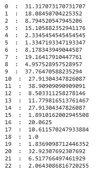
for key, value in class_weights.items():
    print ( key, ' : ', value)
    # Based on https://stackoverflow.com/questions/66501676/how-to-set-class-weights-by-dictionary-for-imbalanced-classes-in-keras-or-tensor

Step-by-step, the procedure is like this: first, we create an empty dictionary called class_weights (Line 1). We then run a for-loop (Lines 2 and 3) to assign the weights to each class. In Line 3, max_samples refers to a pre-calculated value, the maximum number of samples in any one class. In our case, it happens to be 1284, which is the number of samples in the ‘Archie’ class. This value is divided by the number of samples in each class to obtain the class weight for that class. As an example, the ‘Kleats’ class has 41 samples, and so its class weight is 1284 / 41 = 31.3. The ‘Jughead’ class has a far greater number of samples, and so its weight is 1284 / 962 = 1.3.

That’s essentially all that we need to do to get the class weights. If we want to check if we have assigned the weights correctly, we can print out the dictionary (Lines 4 and 5) to get:

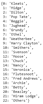
The ‘key’ numbers have been assigned sequentially in the for-loop - note the ‘class_weights[i]’ in the code above. We can check which number corresponds to which class via the ‘inv_index_classes_dict’ created earlier in the notebook, which has for its content:

The only thing that now needs to be done is to pass the class_weights dictionary as an argument while fitting the model:

history = model.fit(
        train,
        validation_data=valid,
        epochs=20,
        callbacks=[stopping, checkpoint],
        class_weight=class_weights
)

Et voilà! We obtain a validation accuracy of around 48%, which is lower than that obtained without class weights, around 56%. Something more interesting is the change in the shape of the training curves:

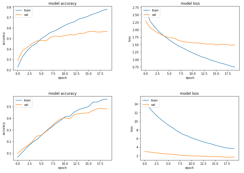
Unweighted model curves on top, weighted bottom

Looking at the model loss curves, we see that for the unweighted model (top), the training loss starts at around 2.75 and drops to around 0.75 after 20 epochs. The weighted training loss (bottom), however, starts at around 15 and remains around 4 at the end of the run. This reflects in a difference in the accuracy curves as well, with a training accuracy of around 78% obtained for the original model after 20 epochs and only 56% for the weighted model. The validation loss, meanwhile, has a similar pattern for both the models, and so the drop in validation accuracy is less pronounced. All this adds up to a far lower degree of overfitting in the weighted model as compared to the original. In other words, class weighting here is also acting as a regularisation technique!

As we are not overfitting after 20 epochs and the validation accuracy appears to have room to rise further, I also created a notebook looking at a run of 50 epochs. We will see the results at the end of this post.

So our original intention was to produce a model which would be roughly equally accurate on the majority and minority classes. How does class weighting fare in that respect? We will come to that, but first a detour.

Last time around, I had described F-scores and how they can be used to quantitatively compare classification models. I may, however, have mistakenly given the impression that F-scores are the only way of doing this, or that they are infallible. Neither is true, and there are in fact plenty of statistical measures that may be used depending on the circumstances. Perhaps one day I will write a blog post going into several of these, but today I will focus on one that is relevant to balanced classification on the ACMC - the Matthews correlation coefficient (MCC).

Matthews correlation coefficient

The Matthews correlation coefficient (MCC), more generally known as the phi coefficient, is calculated for binary classification as:

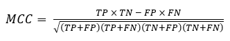
While the F-score ranges from 0 (completely useless model) to 1 (perfection), the MCC ranges from -1 to 1, with a higher score better, and 0 indicating a random model. We can see that, like the F-score, its calculation includes the true positives (TP), false positives (FP) and false negatives (FN). However, unlike the F-score, we also take into account the true negatives (TN). Therefore, a high MCC score is only obtained if a model does well on all four confusion matrix categories. There has been some… work… published… suggesting that the MCC is more reliable and robust than the F-score and other metrics for binary classification, especially for unbalanced datasets, while others contest this. I am not competent enough to arbitrate on this, but at the very least the MCC should be a significant addition to our toolbox, either in addition to or in place of the F-score.

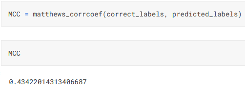
While the MCC can be adapted to multiclass classification via micro- and macro-averaging like the F₁ score, it also has a generalised equation that is given in Wikipedia (as well as articles like this). The formula is rather indimidating, and while it is certainly possible to code it from scratch, a better option may be to use Scikit-learn’s in-built method that can be used for either binary or multiclass classification. The code for this is simplicity itself - we simply import matthews_corrcoef from sklearn.metrics and then pass it the true labels and the predictions:

Results

All right then, let us have a look at the results. The table below compares 3 approaches - using the whole dataset, undersampling, and class weighting - on 7 different criteria. You may want to refresh your memory on the details of the undersampling-min and undersampling-200 approaches, otherwise let’s go!

Before we discuss the results, though, a couple of notes: first, unlike in the previous post, the undersampling-200 approach code looked at here does not use training set augmentations, so as to enable a fairer comparison with the other approaches, none of which use augmentations either. Second, I have bolded the best results for each criterion in the table, but given the stochastic nature of the models, close results may often be flipped, and that is why I have also highlighted values that are close to the best in the table.

Approach	Epochs	RT (s)^a	Train acc. (%)	Val. acc. (%)	Macro-F₁	Micro-F₁	MCC	Code
Whole dataset	20	614	78	57	0.37	0.57	0.51	1
Whole dataset	50	1535	96	60	0.45	0.6	0.55	2
Undersampling-min	50	218	98	31	0.3	0.31	0.28	3
Undersampling-200	50	735	97	46	0.43	0.46	0.43	4
Class weighting	20	618	56	48	0.39	0.48	0.43	5
Class weighting	50	1534	83	58	0.47	0.58	0.53	6

^a: Approx run time in 2022 on Kaggle Notebooks using GPU

Now, looking at the table, a few things stand out. Firstly, for the whole dataset, overfitting is evident even after 20 epochs, and this only increases further after 50. However, the macroaverage F₁ score does show considerable improvement under further training, far more than the micro-average F₁ score does. Intuitively, this would suggest that the model first learns mostly on the majority classes before turning its attention towards the minority classes in an effort to raise the accuracy further.

In case of undersampling, using the minimum number of samples per class makes for very fast training due to the much-reduced number of samples. That’s all that it has going for it, though - while training accuracy approaches 100%, the other parameters are very bad indeed. The undersampling-200 approach fares much better, although compared with using the whole dataset, again the only area it does better is the shorter run time. The MCC is considerably lower than for the whole dataset, and the macro-F₁ score slightly inferior, which means that our hope of building a more equitable model hasn’t really come to pass using undersampling.

Class weighting, as we saw earlier, narrows the overfitting considerably, which is a plus. The remaining results, however, are merely comparable with using the full dataset, rather than an improvement. The fact that the training accuracy still has upward room may mean that further training will improve the other values, but this would of course be at the cost of increased training time.

A final comment. We see that the MCC tend to lie between the micro- and macro-F₁ scores, and rise and fall in tandem with them. For this dataset, therefore, it does not appear to provide any novel insights. It would be unfair to draw any conclusions based on this alone, however, and so I will continue using the MCC in conjunction with the F₁ score, and see if they diverge in future studies, and what such divergence could mean.

Conclusion

So far we have tested two approaches for developing a classifier that is similarly accurate on the different classes of the ACMC dataset. Unfortunately, neither undersampling nor class weighting were able to significantly improve upon simply using the original dataset. Perhaps oversampling will do the trick? Or maybe a combination of different options? We shall see…for now, bye!