9. Diving into the Archie Comics Multiclass dataset
Categories:
Tags:
TensorFlow 2, Keras, Matplotlib, Seaborn, PIL, Pandas, Scikit-learn, Confusion Matrix
Hi there! Last time we had a brief look at the Archie Comics Multiclass (ACMC) dataset that I created, and which can be found here. In this post, let us look at the dataset in a little more detail, and then do some simple modelling on it.
A look at the images and their distribution
You can find a notebook looking at the images here. The first part of the notebook looks at two images from each of the folders (as a reminder, there are 23 folders, for each of the 22 characters + ‘Others’), but as we already saw something similar in the previous post, let us move on to one of the aspects that I think makes this dataset really interesting- the class distribution. The code below first creates and populates two lists, one for the class names and the other for the number of samples per class, by walking through all the image folders. We can then create a Pandas dataframe from these lists, and plot them in a bar plot using Seaborn.
samples_per_class = []
classes = []

directory=os.listdir('../input/archie-comics-multi-class/Multi-class/')
for each in directory:
    currentFolder = '../input/archie-comics-multi-class/Multi-class/' + each
    count = sum(len(files) for _, _, files in os.walk(currentFolder))
    samples_per_class.append(count)
    classes.append(each)

df = pd.DataFrame(list(zip(classes, samples_per_class)),
                   columns =['Classes', 'Samples per class'])

rcParams['figure.figsize'] = 15,8

sns.barplot(data=df, x = 'Classes', y = 'Samples per class')
ticks = plt.xticks(rotation=45)
All right, so let us see what the class distribution looks like…
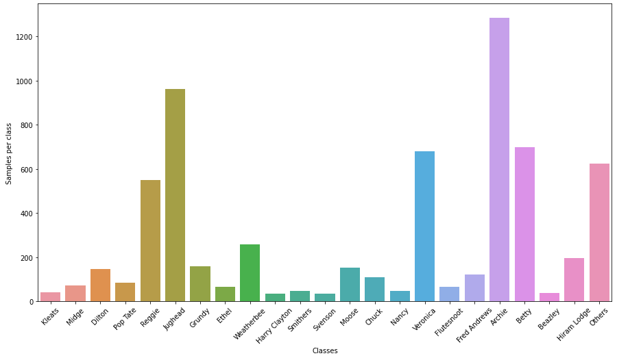
Image 1: Class distribution of ACMC images
Wow, that’s quite something, right? We see that there are nearly 1300 Archie images, while the other major characters, and ‘Others’ have plenty of samples as well (>500 each). On the other hand, some of the minor characters have less than 50 samples apiece. This imbalance is a challenge, but I think is quite representative of the real world, where data is unlikely to be neatly balanced.
But the imbalance is not restricted just to the number of images per class - let us see what the image size distribution looks like. We can use Pillow to get the size of every image, store these in a list of tuples, and then make a scatter plot. Along the way, we also check the median and mean of the tuples.
sizes = []
for each in directory:
    currentFolder = '../input/archie-comics-multi-class/Multi-class/' + each

    for i, file in enumerate(os.listdir(currentFolder)):
        fullpath = currentFolder+ "/" + file
        img = Image.open(fullpath)
        sizes.append(img.size)

np.median(list(dict(sizes).values()))
# from https://stackoverflow.com/questions/31836655/using-numpy-to-find-median-of-second-element-of-list-of-tuples

np.mean(list(dict(sizes).values()))

rcParams['figure.figsize'] = 10,6

# https://stackoverflow.com/questions/47032283/how-to-scatter-plot-a-two-dimensional-list-in-python
plt.scatter(*zip(*sizes))
plt.show()
This plot looks like this:
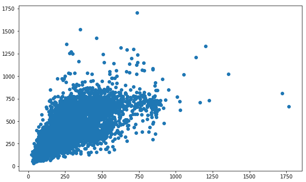
Image 2: Size distribution of ACMC images
There are two things noticeable here. Firstly, the images have a wide size distribution, with the smallest being smaller than 100 pixel x 100 pixel, and the largest exceeding 1000 pixel by 1000 pixel. The code above gives us a median of 437 and a mean of 470.5. The second thing is that the images are far from being square. As computer vision (CV) models like to be fed images that are similarly sized and square-shaped, it is clear that image processing may be key to maximising image recognition accuracy on this dataset.
We can wind up this section with a look at some random images. The exact images displayed will differ every time the notebook is run, but will in general look like this:
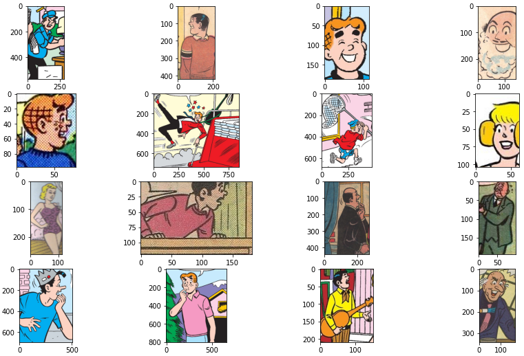
Image 3: A look at random ACMC images
The difference in the image quality, shapes, centering, etc. is obvious from these images. Also, as expected, the main characters and ‘Others’ dominate the images. Less obvious in this subplot is the difference in the image sizes, unless we look at the axes, some of which go beyond 800 while others stop below 100.
All right then, let’s get our hands dirty by doing some modelling on the data!
Simple ResNet models
We will do some more intricate modelling on this data in later posts, but for now, let us make a simple ResNet50-based model on it. I have published the code for this here. The most important parts are given below:
batch_size = 8

train = tf.keras.preprocessing.image_dataset_from_directory(
        path,
        labels="inferred",
        label_mode="categorical",
        class_names=classes,
        validation_split=0.2,
        subset="training",
        shuffle=True,
        seed=123,
        batch_size=batch_size,
        image_size=(256, 256),
    )

valid = tf.keras.preprocessing.image_dataset_from_directory(
        path,
        labels="inferred",
        label_mode="categorical",
        class_names=classes,
        validation_split=0.2,
        subset="validation",
        shuffle=True,
        seed=123,
        batch_size=batch_size,
        image_size=(256, 256),
    )

stopping = tf.keras.callbacks.EarlyStopping(
            monitor="val_accuracy",
            min_delta=0,
            patience=5,
            verbose=0,
            mode="auto",
            baseline=None,
            restore_best_weights=False,
        )

checkpoint = tf.keras.callbacks.ModelCheckpoint(
            "best_model",
            monitor="val_accuracy",
            mode="max",
            save_best_only=True,
            save_weights_only=True,
        )

base_model = tf.keras.applications.ResNet50(weights=None, input_shape=(256, 256, 3), classes=num_classes)

inputs = tf.keras.Input(shape=(256, 256, 3))
x = tf.keras.applications.resnet.preprocess_input(inputs)
x = base_model(x)
model = tf.keras.Model(inputs, x)

model.compile(
                optimizer=tf.keras.optimizers.Adam(learning_rate=0.0001),
                loss=tf.keras.losses.CategoricalCrossentropy(),#from_logits=True),
                metrics=["accuracy"]
            )

loss_0, acc_0 = model.evaluate(valid)
print(f"loss {loss_0}, acc {acc_0}")


history = model.fit(
                train,
                validation_data=valid,
                epochs=20,
                callbacks=[stopping, checkpoint]
        )

model.load_weights("best_model")

loss, acc = model.evaluate(valid)
print(f"final loss {loss}, final acc {acc}")

# summarize history for accuracy
plt.plot(history.history['accuracy'])
plt.plot(history.history['val_accuracy'])
plt.title('model accuracy')
plt.ylabel('accuracy')
plt.xlabel('epoch')
plt.legend(['train', 'val'], loc='upper left')
plt.show()
# summarize history for loss
plt.plot(history.history['loss'])
plt.plot(history.history['val_loss'])
plt.title('model loss')
plt.ylabel('loss')
plt.xlabel('epoch')
plt.legend(['train', 'val'], loc='upper left')
plt.show()
Briefly, what the above code does first is generate training and validation TensorFlow datasets with a 80:20 split. Note that since we do not have a pre-existing training-validation split, i.e. separate folders for training and validation, we use the image_dataset_from_directory util instead of the more customary flow_from_directory ImageDataGenerator. Next, we define and fit a ResNet50 model, saving the model with the best validation accuracy via a checkpoint callback. We also provide an early stopping callback, with a ‘Patience’ of 5, i.e., the model will stop running if the validation accuracy doesn’t improve over 5 epochs. The remaining parameters are fairly standard. After the run, we plot the model accuracy and loss over the epochs, which look like this:
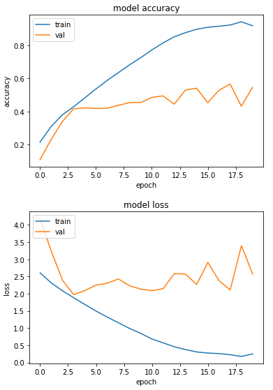
Image 4: Accuracy and loss of ResNet50 model without pre-trained weights
We can see that the plots show definite overfitting, with a divergence between the training and the validation curves. The other noteworthy feature is the jaggedness of the curves, one reason for which may be the small batch size (8) employed.
The maximum validation accuracy obtained in the above run is around 57%. This made me wonder - what if I started with Imagenet weights for the ResNet instead of no weights? I made another notebook on that here. The main change is that for using the Imagenet weights, the model head needs to be changed, which I did as per this - the modified portion of the code is shown below, while the rest remains unchanged.
# construct the head of the model that will be placed on top of the
# the base model
headModel = base_model.output
headModel = AveragePooling2D(pool_size=(7, 7))(headModel)
headModel = Flatten(name="flatten")(headModel)
headModel = Dense(256, activation="relu")(headModel)
headModel = Dropout(0.5)(headModel)
headModel = Dense(num_classes, activation="softmax")(headModel)
# place the head FC model on top of the base model (this will become
# the actual model we will train)
model = Model(inputs=base_model.input, outputs=headModel)
# loop over all layers in the base model and freeze them so they will
# *not* be updated during the training process
for layer in base_model.layers:
    layer.trainable = False
And we obtain a maximum validation accuracy of…56%…in other words, it appears to make no difference whether we use the Imagenet weights or not. This, however, is only true if we look just at the highest validation accuracy. Looking at the training curves gives a slightly different picture.
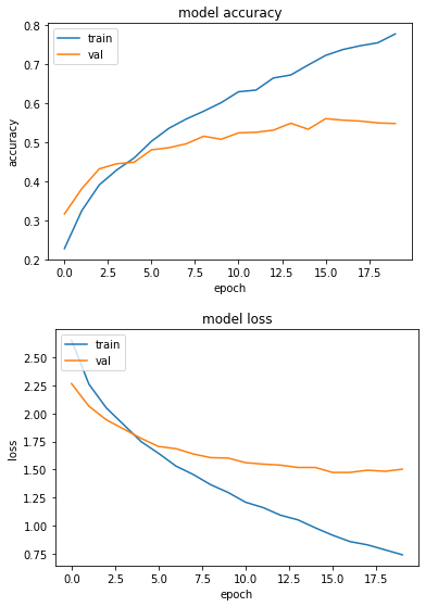
Image 5: Accuracy and loss of ResNet50 model with Imagenet weights
We can see that the curves are much smoother, implying that the training is a lot more stable - a feature not to be underestimated while training a small unbalanced dataset - or any dataset for that matter. On the other hand, the issue of overfitting remains, but that is understandable given the class imbalance. We will see later if we can do something about this.
Effect of image size on validation accuracy
One point that I did not comment on earlier was the image size we fed into the ResNets. If you see the code above, we used an input size of 256 x 256. I selected this size because, looking at Image 2, it is clear that the vast majority of images are larger than this, and it is generally preferable to downscale images to smaller sizes than upscale them by stretching the pixels.
Nevertheless, it is worth taking a look at what effect changing the image size has on accuracy, which is what I did in this notebook. Essentially, I made a list of three numbers - 128, 256 and 512 - and ran these as image sizes in a for-loop. The maximum validation accuracies I got were revealing - 0.43 for 128 x 128, 0.51 for 256 x 256, and 0.63 for 512 x 512. Why is the 256 x 256 accuracy lower than what we got earlier? Mainly because the early stopping kicked in on this particular run and halted the run after only 10 epochs, which is why the absolute numbers must be taken with a pinch of salt. The trend, however, is what is interesting, as we see a clear increase in validation accuracy with image size. Why would this be the case? Well quite simply, all other things equal, larger images have higher resolution, making it possible for the CV model to learn from details that are lost when the image is shrunk. This is in line with results obtained, for instance, in this paper, which looked at the effect of varying image resolutions from 32 x 32 to 512 x 512 and found the best results at the highest resolution.
If this is the case, then why did I not try an even higher resolution? Actually, I did try running the model at 1024 x 1024, and ran into a ‘Resource Exhausted Error’. Essentially, trying to load images of this size into memory results in a memory error. Resolving that would require making other changes in the code. One option would be reducing the batch size - but that is already just 8, and reducing it further would further increase the volatility that we have already seen in the training curves. Another would be employing a smaller model - but then the comparison with the other image sizes modelled with ResNet50 would not be apples and apples. A third would be to upgrade the system configurations…not really possible in a Kaggle notebook!
.
.
.
However, even if we could run at 1024 x 1024, we would be unlikely to see much improvement. Why? Remember that we saw that the median image size was 437, while the mean was 470.5. Increasing the size much beyond this would likely be unhelpful, since, as noted here, increasing image sizes beyond their original dimensions stretches image pixels, impacting the ability of models to learn key features like object boundaries. Therefore, ‘the larger the better’ is only true for image size up to a point, with accuracies often dropping when image size is further increased. And finally, even if the accuracy doesn’t drop, one still needs to be consider if the 64-fold increase in memory requirement and processing time caused by an 8-fold increase in image size (from 128 x 128 to 1024 x 1024) will really be worth it…
So, in short, 512 x 512 seems like a good image size, giving high validation accuracy without crashing our system. This image size does take considerably longer to train, though, than 128 x 128 - a 10 minute run for 128 x 128 may become a 160 minute run for 512 x 512. Given this, progressive resizing, a concept introduced by Jeremy Howard at FastAI, may be a good way to get great accuracies while keeping training times reasonable. As mentioned in that link,
One of our main advances in DAWNBench was to introduce progressive image resizing for classification – using small images at the start of training, and gradually increasing size as training progresses. That way, when the model is very inaccurate early on, it can quickly see lots of images and make rapid progress, and later in training it can see larger images to learn about more fine-grained distinctions.
For now, we will park this idea, since the aim of this post is to keep things simple, and revisit the concept in a later post.
The elephant in the room
All right, we have talked quite a bit about validation accuracies and image sizes, but haven’t really mentioned one thing that really is important for a dataset as unbalanced as this - how good is the model at identifying each character? In other words, is the high accuracy just because it has learnt to recognise the main characters, or is it more well-rounded? Let’s find out!
Since we saw that using the Imagenet weights gives smoother training curves and using an image size of 512 x 512 increases validation accuracy, I made yet another notebook, this time using these parameters. The maximum validation accuracy obtained? 0.63! Yay! But that’s not what we are really interested in here. We are more into the information presented in the ‘confusion matrix’. A confusion matrix is a great tool to see at a glance how a machine learning algorithm has performed on a class-level, i.e., how many examples of each class it has correctly classified, and into which classes the incorrect results fall. A simple example is given by Scikit-learn for the Iris dataset:
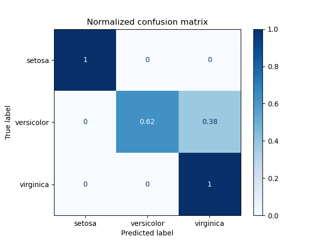
Image 6: Scikit-learn's example of a confusion matrix on the Iris dataset
We see here in the normalised confusion matrix that perfect results were obtained for the setosa and virginica irises, while for the versicolor, 62% were correctly classified, the rest all being misclassified as virginica.
For the final run on our dataset, the normalised confusion matrix (created using Scikit-learn) looks like the image below. (Note: the image looks much better on Firefox than Chrome, due to a well-known problem Chrome has with downscaling images. If needed, you can open the image in a new tab and zoom it to make it easier to read.)
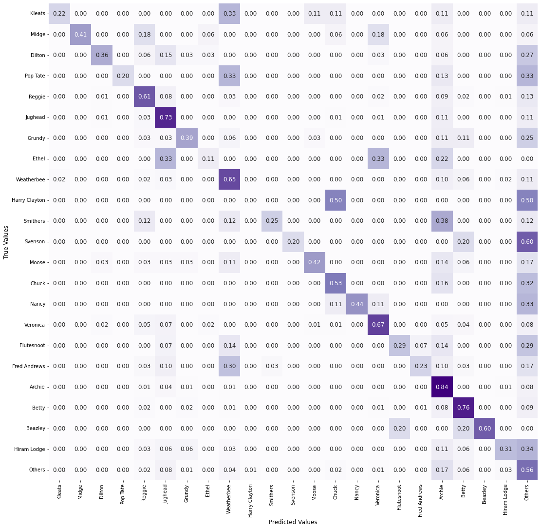
Image 7: Normalised confusion matrix
Hmmm, we see that the performance is all over the place, and that for some classes, the results are really quite poor. We also see that the model has put some examples from almost every class into ‘Others’, which makes sense if you think about it - if the model is sure that an example is Grundy or Moose, it goes into that category, while any it is unsure of goes into the catch-all bin of ‘Others’.
To better understand the model performance, however, we may want to also have a look at the non-normalised confusion matrix. Here it is:
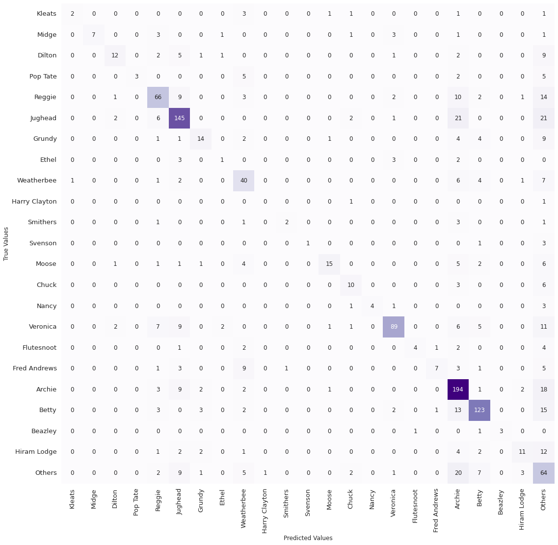
Image 8: Non-normalised confusion matrix
To get why this is important, have a look at the Harry Clayton class. The normalised confusion matrix was disappointing for this class, as it showed that the model did not make a single accurate prediction on this class. Image 8, however, shows that there were only two images of this class in the validation set! The 0% true positive rate for this class is not, therefore, as shocking as it might first seem. The random manner in which the validation set is selected means that several of the smaller classes may be under-represented even more severely in the validation set than they had been in the original dataset, which is clearly the case here for Harry Clayton. Other runs had given a 100% true positive rate for the same class! This means that for the minor character classes, it is not merely difficult to model them but also hard to quantify the model performance on them.
A picture may help demonstrate the effect of class size on the classification performance more vividly. The excellent top-rated answer (not the accepted answer) on a Stackoverflow question shows how to get the true positives (Archie predicted as Archie), true negatives (non-Archie predicted as non-Archie), false positives (non-Archie predicted as Archie) and false negatives (Archie predicted as non-Archie) from a confusion matrix. Let us just deal with the true positive rate (TPR) (also called sensitivity or recall) for now, i.e., what fraction of, say, Ethel pix were correctly predicted as Ethel. The code below calculates the TPR for each class, makes a Pandas dataframe out of these, and then uses that dataframe to create a Seaborn regression plot.
FN = cm.sum(axis=1) - np.diag(cm)
TP = np.diag(cm)
# from https://stackoverflow.com/questions/31324218/scikit-learn-how-to-obtain-true-positive-true-negative-false-positive-and-fal
TPR = TP/(TP+FN)

df_from_arr = pd.DataFrame(data=[samples_per_class, TPR]).T
df_from_arr.rename(columns={0: "No. of samples", 1: "True positive rate"}, inplace = True)
df_from_arr.index = classes
df_from_arr["No. of samples"] = df_from_arr["No. of samples"].astype(int)
df_from_arr["True positive rate"] = df_from_arr["True positive rate"].round(2)

sns.regplot(data=df_from_arr, x="No. of samples", y="True positive rate")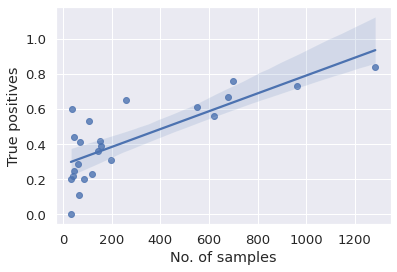
Image 9: True positive rate versus number of samples in class
We see that there is plenty of scatter towards the left-hand side of the plot, with some minor classes having a very low true positive rate and others very high values. We have already seen one possible cause of this - the fact that random selection means that there may be few examples of the classes in the training or validation sets. Another may be that the image quality or other factors could make certain classes easier to classify. And finally, some characters may simply be easier to recognise than others!
On the whole, though, the trend is clear - there is a clear upward trend, indicating that the characters with more images available are classified more accurately than those with fewer, which is what we would expect. For Archie pix, we have a TPR of 0.84, which is quite impressive, while Jughead and Betty also have a TPR of over 0.7, Veronica and Reggie getting 0.67 and 0.61 respectively.
Does it matter?
We see that the major classes contribute heavily towards the overall accuracy of 0.63. Is that something we should be happy about? Well, that depends on what we want! If we are trying to build a classifier that will perform well on a randomly selected page from an Archie comics digest, we should be quite happy with what we have done so far. The odds of getting an Archie or a Jughead image, as opposed to a Beazly or Kleats image, in a random Archie comics panel is actually even higher than indicated by this dataset. So it makes sense for us to build a classifier that would work well on the major classes. Think of it this way - if you are building a dog image classifier, you would probably want your model to work well on German Shephard or Golden Retriever images, even if it gets the occasional Azawakh or Lagotto Romagnolo wrong.
If, on the other hand, we want a classifier that will work roughly equally well on every class, then our current approach is clearly not working. What can we do to sort this out? We shall see next time, when we discuss the different approaches for handling unbalanced datasets. For now, ciao!