ACMC - Undersampling and F-scores | Agneev’s DS/ML lab book

Categories:

Machine Learning Computer Vision Python Metric

Tags:

TensorFlow 2, Keras, Matplotlib, Seaborn, Pandas, Scikit-learn, F-score

[Edit: This post expands on a previously published version, with a description of F-scores and an alternative undersampling approach added.]

Hello! It’s been a long time since my previous post, as I have had plenty to do, professionally and personally, since then. This also means that this post will be shorter than I had originally planned. Last time I left off saying that we would be looking at different approaches for handling unbalanced datasets, but today we will only look at one such approach - the rest (hopefully) coming soon!

So, as a brief reminder, we are dealing with the Archie Comics Multiclass (ACMC) dataset that I created and placed here. We have already seen how a simple model can get a decent validation accuracy of around 56%, at the cost of a) overfitting, and b) having a far higher true positive rate (or recall) for the classes having more samples (i.e. the majority classes) in the unbalanced dataset. The overfitting we leave aside for the moment, but what if we need a model that is approximately equally accurate for every class? For this, we need to overcome the class imbalance, such as via…

Undersampling

Since some of the classes having more samples than others is our issue, the first way of handling it would be to simply make the number of samples the same. This could be done either by reducing the number of samples considered in the majority classes (undersampling) or increasing the number of samples in the minority classes via duplication or synthetic sampling (oversampling). We will look at oversampling in a later post, but how do we go about undersampling?

The simplest thing to do is to look at the minimum number of samples that are present in every class and just take that many images from each class. In other words, we reduce all the columns in the figure below to the red line showing the level of the minimum samples class (Svenson). This method ensures that every class has the same number of samples, at the cost of discarding a large number of samples from the majority classes.

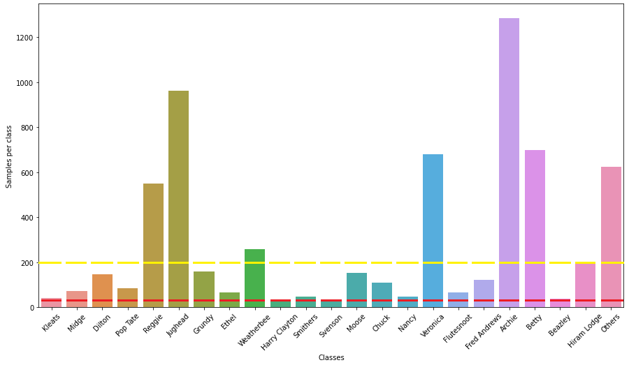
An alternative is to fix a particular threshold, say 200 samples, and remove the excess samples for the classes that have a higher number of samples. This is denoted by the yellow line in the figure. In this case, a degree of imbalance persists among the classes, but to a much lesser extent than in the original dataset, and we get to train with more samples than using the minimum samples approach.

Let’s look at both approaches in turn.

Minimum samples approach

Now, I mentioned the ‘simplest thing to do’ above, but I found it surprisingly hard to actually carry it out in TensorFlow. After trying different methods, I finally decided that using the flow_from_dataframe function of Keras is the best way to go about things. It’s not perfect - it is a function of Keras’ ImageDataGenerator, which is deprecated. Still, this method allows us to quickly look at the effect of undersampling on the results without having to actually create new directories containing fewer images, etc., and so we’ll stick with this for now. The full code is on Github here - let’s look at the important parts.

First, let’s create and populate lists with the names of the classes, number of samples per class, and the image filenames:

samples_per_class = []
classes = []
file_names = []

directory=os.listdir('../input/archie-comics-multi-class/Multi-class/')
for each in directory:
    currentFolder = '../input/archie-comics-multi-class/Multi-class/' + each
    count = sum(len(files) for _, _, files in os.walk(currentFolder))
    samples_per_class.append(count)
    classes.append(each)

    for i, file in enumerate(os.listdir(currentFolder)):
            fullpath = currentFolder+ "/" + file
            file_names.append(fullpath)

min(samples_per_class)

The line at the end of the above code will show that the minimum number of samples in each class is 33. Now to go about undersampling. To do this, first let’s create a list of 33 filenames per class. There are various ways of doing this, but the code below is what I have gone for.


1
2
3
4
5
6
7
8

small_ds = []

for each_class in classes:
    trial_list = []
    for name in file_names:
        if re.search(f'{each_class}', name):
            trial_list.append(name)
    small_ds.append(random.sample(trial_list, min(samples_per_class)))

This code deserves a bit of explanation, and so I have added line numbers to the code block above to make it easier to understand. Essentially, after creating an empty small_ds list (Line 1), we run a for-loop for each class populating this list (Line 3). The for-loop itself works like this: consider any class, for instance ‘Jughead’. We create a new empty trial_list (Line 4), then, using a nested for-loop (Line 5), scan through the file_names list we created earlier. Using a regular expression (Line 6), we select the filenames containing ‘Jughead’. These file names are added to trial_list (Line 7). At the end of the nested for-loop, trial_list contains all the filenames containing ‘Jughead’ in them. Exiting the nested for-loop, we add 33 randomly selected ‘Jughead’ filenames from trial_list to the small_ds list (Line 8). We then move to the next class in the outer loop (Line 3), with a new empty trial_list being created (Line 4), and so on. At the end, therefore, we get a list containing 33 randomly selected filenames for each of the 23 classes.

Let us see whether we have created the small_ds properly. First, the length:

print(len(small_ds))
print(len(small_ds[0]))
print(len(small_ds)*len(small_ds[0]))

The results of the above print statements are 23, 33, and 759. In other words, we have created a 2D list with dimensions 23*33. Handling this list might be easier if it’s 1D, so let’s flatten it.

small_ds=list(np.concatenate(small_ds).flat)
print(len(small_ds))

The length is now 759, indicating we have successfully obtained a 1D list containing all the filenames. We can peek into this list and see:

The list, we see, contains the complete filenames selected randomly. Let us now make a Pandas dataframe out of this list.


1
2
3
4
5
6
7
8
9
10

files_df = pd.DataFrame(index=range(0, len(small_ds)),columns = ['Class'])

start = 0
end = min(samples_per_class)
for each_class in classes:
    files_df.iloc[start:end] = each_class
    start = end
    end = end + min(samples_per_class)

files_df['Class'] = files_df['Class'].astype('str')

Above, we first create an empty Pandas dataframe with an index between 0 and 759 and a solitary ‘Class’ column (Line 1). We now need to fill up this ‘Class’ column - I have used a quick and dirty method in the code above, but this, as we will see, is not suitable for a general case. This method is simply using a for-loop (Lines 5-8) so that rows 0-32 containing the first class name, 33-65 the second, and so on.

The small_ds dataset is then added as a new column ‘Files’:

files_df['Files'] = small_ds

We now see the files_df dataframe has the class names and the file names:

Now, during my first run, I left things like this and moved on to modelling - this is an error! Try and figure out why, and we will return to the question a little later

Model run

So the next step is to create training and validation generators with a 80:20 training-validation split. We can as usual apply a range of image augmentations to the training set here (as explained in my earlier post).

datagen=ImageDataGenerator(validation_split=0.2)

batch_size = 8

train_generator=datagen.flow_from_dataframe(
dataframe=files_df,
directory=None,
x_col='Files',
y_col='Class',
subset="training",
batch_size=batch_size,
seed=42,
shuffle=True,
class_mode="categorical",
# rotation_range=30,
# width_shift_range=0.2,
# height_shift_range=0.2,
# brightness_range=(0.5,1.5),
# shear_range=0.2,
# zoom_range=0.2,
# channel_shift_range=30.0,
# fill_mode='nearest',
# horizontal_flip=True,
# vertical_flip=False,
target_size=(256,256))

valid_generator=datagen.flow_from_dataframe(
dataframe=files_df,
directory=None,
x_col='Files',
y_col='Class',
subset="validation",
batch_size=batch_size,
seed=42,
shuffle=True,
class_mode="categorical",
target_size=(256,256))

We can then run the model, with the usual callbacks. Initially, let us have a patience value of 15 epochs for the early stopping, and run it for 50 epochs. The image sizes I used were 256 x 256, the base value used last time. The first results look like this:

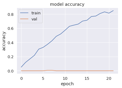
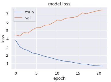
Hmm…strange. The training accuracy and loss are fine, but the validation accuracy remains virtually at zero, while the validation loss actually rises relentlessly. Clearly something is wrong…

Remember I said earlier that creating the dataframe and moving directly to modelling was an error? Well, what this has resulted in is a complete mismatch between the training and validation sets. In Keras, “validation_split = 0.2” leads to the bottom 20% of the input data being designated as the validation set while the upper 80% is the training set. This means that here, the training set consists of all the classes that appear in the upper portion of the files_df dataframe (Kleats, Midge, Dilton, etc.), while the bottom (Beazley, Hiram Lodge, Others…) becomes the validation set. No wonder then that the results are so poor, since the model is being trained on one set of classes and validated on another set!

We therefore add a crucial line of code prior to creating the generators:

files_df = files_df.sample(frac=1, random_state=1).reset_index()

The above line of code is explained well here and so I won’t go into the details, but in short, it shuffles the rows of the dataframe so that our training and validation sets now receive a mix of classes. If we see the last 10 rows of the dataframe, we now see:

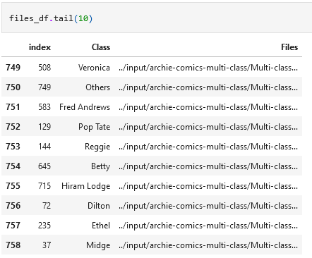
That’s better…the different classes are now randomly arranged. We see that the original indices have been added as a column, which we can drop if we choose. Anyway, if we run the model again, we now get:

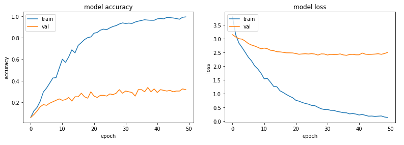
We see that the validation accuracy and loss now look more familiar (and appropriate). Let us recap a sentence from the start of this post, however.

A simple model can get a decent validation accuracy of around 56%, at the cost of a) overfitting, and b) having a far higher true positive rate (or recall) for the classes having more samples (i.e. the majority classes) in the unbalanced dataset.

In the simple model, we got the validation accuracy of 56% after 20 epochs. Here, after 50 epochs we managed around 33%. A cursory glance at the training curves shows that the overfitting problem has got worse. However, these things are not really surprising - we are using far fewer samples in this run, so understandably the accuracy figures suffer and overfitting occurs. The reason we experimented with undersampling in the first place was not to improve the validation accuracy or solve overfitting, but to make the results more equitable across the classes. Have we at least achieved that? Let us look at the confusion matrix. (Note: the image looks much better on Firefox than Chrome, due to a well-known problem Chrome has with downscaling images. If needed, you can open the image in a new tab and zoom it to make it easier to read.)

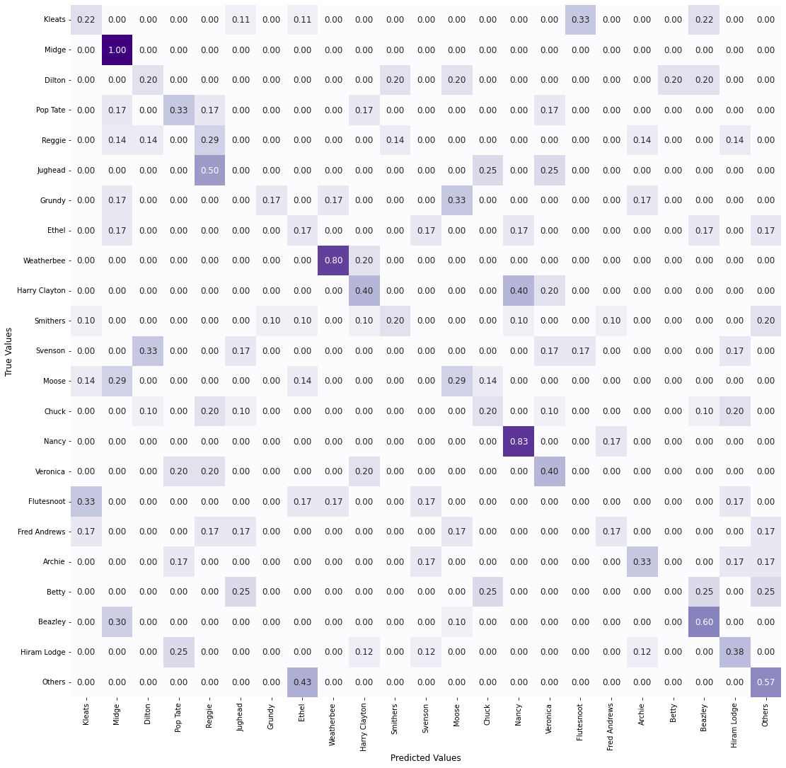
Viewed one way, the problem of the majority classes getting higher true positive rates has been resolved - the results for Archie, Jughead, etc. are pretty average now. On the other hand, several classes still perform much better or worse than average. Why is this? Well, one reason can be divined from looking at the absolute numbers in the confusion matrix:

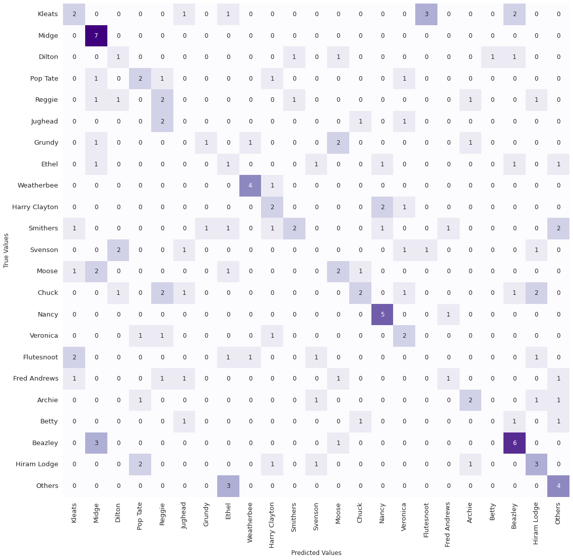
We see that some classes have as few as 4 samples in the validation set, and in general, the number of samples are too few to make a reasonable judgement about how good the model is for any class, considering both the heterogeneity of the dataset and the stochastic nature of ML models. Other factors for why some classes show a higher true positive rate might be some characters being easier to identify, the validation images more closely resembling the training figures for these classes, etc. In any case, our stated goal of achieving an even recognition of all the classes thus remains unaccomplished…

Arbitrary threshold approach

As I said near the start of this post, an alternative to the minimum samples approach would be to fix a particular threshold and discard the excess samples for the majority classes. This threshold is somewhat arbitrary, but looking at Image 1, we see that 200 samples seems to be a pretty good value to pick. If we choose a smaller number, say 100, then we will be discarding a lot of images, since most of the classes have more than 100 images. On the other hand, a threshold of 300 or above will again result in an excess of samples from the majority classes, since only these have more than about 250 images. 200 seems to be a good compromise number, and so let’s go with this (complete code here).

The procedure is similar to that we saw earlier, with one critical difference. Remember that we had used a for-loop to fill the ‘Class’ column with 33 rows of each samples in files_df? So that we got something like this?

We can’t use this now, since we don’t have the same number of samples for each class. Instead, we will have to do things the hard way and get the class names from the file names. The code for this is:


1
2
3
4
5
6
7
8
9
10
11

files_df = pd.DataFrame(index=range(0, len(small_ds)),columns = ['Files'])

files_df['Files'] = small_ds

files_df['Class'] = files_df.Files.str.extract(r'Multi-class/(.*?)/', expand=True)

files_df = files_df.sample(frac=1, random_state=1).reset_index(drop=True)

pd.set_option('display.max_colwidth', None)

files_df.tail(10)

In Line 1 above, we create the files_df dataframe, but use ‘Files’ as the original column now. We then populate the column with the small_ds list as earlier (Line 3). After this, we use a regular expression to extract the class name from the file name (see this) and store this in a newly created ‘Class’ column (Line 5). Line 7 randomly shuffles the rows as before, only this time I am dropping the original indices instead of adding them as a new column. Line 9 is optional, but important here. Pandas typically limits column width and only displays the first few characters of every row in the column. However, if we want to check whether the class names have been correctly selected, we need to see the end of the file names, which we can do by setting the maximum column width to ‘None’. Finally, looking at the last 10 rows of the dataframe (Line 11), we see:

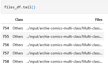
Yes, this looks fine. We also see that the number of rows has now increased to 2807 (starting from 0), so we are now using a much greater proportion of our original dataset. We can then go on with the modelling as usual, finally getting a validation accuracy of around 50% from 50 epochs (after applying some augmentations to the training set, check out the complete code for that).

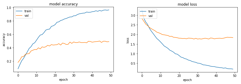
Once again we see the overfitting persisting, but once again, that’s not our concern here. What does the confusion matrix look like?

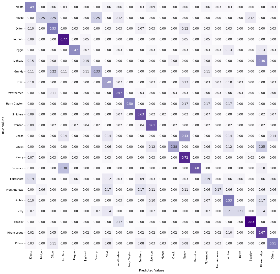
Hmm. This certainly appears better than the minimum samples approach. Is it better than that of the original dataset, however? If so, by how much? Better enough to justify the loss in validation accuracy?

So far we have been handling these things qualitatively. If we are to answer the above questions, however, we need to be more quantitative. Using just accuracy won’t work - we need a metric that can compare models taking into account not only the predictions that the models got correct but also those they got wrong. Enter the…

F-score

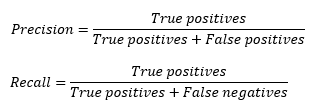
As Wikipedia says, the F-score is a measure of accuracy calculated using precision and recall. What are these terms?

Precision (also called positive predictive value) is the ratio of true positives (TP) to all positive predictions (true positives + false positives (FP)). Recall (also called true positive rate or sensitivity) is the ratio of true positives to actual positives (true positives + false negatives (FN)). They are calculated as per:

We can better understand the above equations with a concrete example. Let us look at the absolute numbers obtained for the Archie class in the confusion matrix for the 200 sample threshold undersampling.

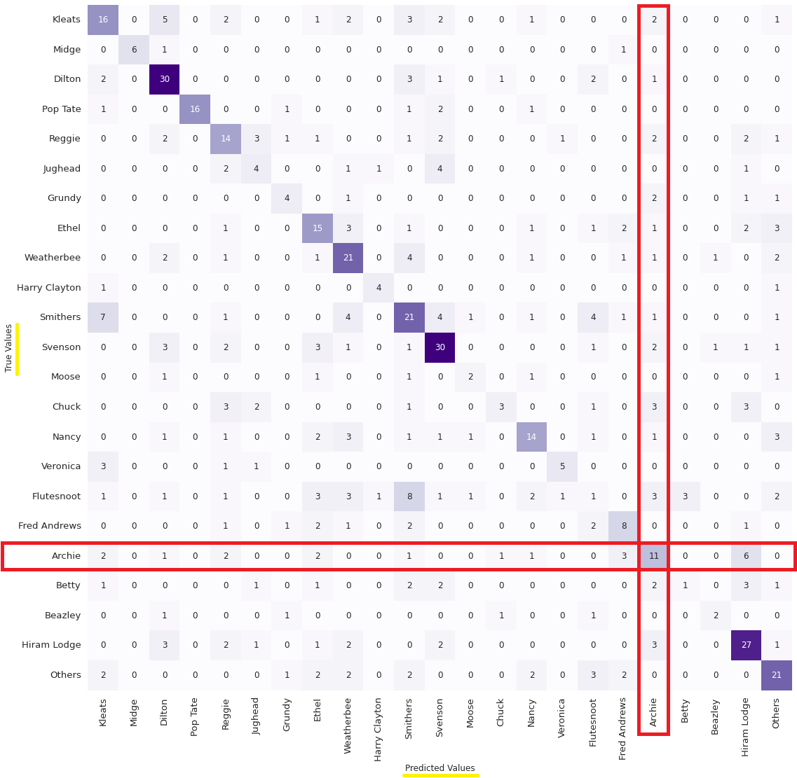
Adding up the numbers for ‘True Values’, we see that there are a total of 30 Archie images in the validation set. Of these, our model has correctly predicted only 11 (True Positives), meaning that 19 images were incorrectly classified as belonging to other classes (False Negatives). The recall, therefore, is 11/(11+19) = 0.37.

What about the precision? We see that no fewer than 35 images had been identified as Archie (adding up the ‘Predicted Value’ numbers), of which, again, only 11 are correct predictions (True Positives). The remaining 24 are therefore False Positives. The precision is 11/(11+24) = 0.31.

OK, so now that we have the precision and recall values, how do we get the F-score? There are actually various ways of doing this, giving different importances to precision and recall, but the most widely used is the F₁ score. This is defined as the harmonic mean of precision and recall:

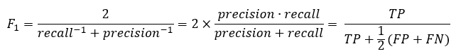
The F₁ score for the Archie class is thus 2 * (0.31 * 0.37) / (0.31 + 0.37) = 0.34.

Is this a good performance? No! F-scores range between 0 and 1, with a higher number indicating a better performing model. At least for the Archie class, therefore, our model hasn’t been brilliant. What about its overall performance, though?

F-score averaging

One thing that I have not mentioned yet is that the F-score is defined for binary classification. The example we looked at above was essentially ‘Archie’ versus ‘non-Archie’, a binary classification problem. How do we adapt the F-score to multiclass classification then? Simply by taking the average of the F-scores for all the classes…but how do we take the average?

The two most widely used F-score averages are the micro- and the macro-averages. These can again be better understood by concrete numbers, so let us first tabulate the TP, FP, TN (true negative), FN and F1 values for all the classes.

Class	True positives	False positives	True negatives	False negatives	F₁ score
Kleats	16	20	506	19	0.45
Midge	6	0	553	2	0.86
Dilton	30	21	500	10	0.66
Pop Tate	16	0	539	6	0.84
Reggie	14	20	511	16	0.44
Jughead	4	8	540	9	0.32
Grundy	4	5	547	5	0.44
Ethel	15	20	511	15	0.46
Weatherbee	21	23	503	14	0.53
Harry Clayton	4	2	553	2	0.67
Smithers	21	32	483	25	0.42
Svenson	30	21	494	16	0.62
Moose	2	3	551	5	0.33
Chuck	3	3	542	13	0.27
Nancy	14	11	521	15	0.52
Veronica	5	2	549	5	0.59
Flutesnoot	1	16	513	31	0.04
Fred Andrews	8	10	533	10	0.44
Archie	11	24	507	19	0.34
Betty	1	3	544	13	0.11
Beazley	2	2	553	4	0.4
Hiram Lodge	27	20	499	15	0.61
Others	21	19	505	16	0.55
Total	276	285	12057	285	nan

The macroaverage F₁ is simply the mean of the F₁ values for all the classes. In this case, the mean of the F₁ score column comes to 0.47, and this is the macroaverage F₁ score.

The microaverage F₁ score, on the other hand, is calculated using the sum of the TP, FP and FN values. Here, the microaverage F₁ = 276 / (276 + 1/2 * (285 + 285)) = 0.49.

We can see that the macroaverage F₁ score gives equal weightage to every class, regardless of the class sample size. The microaverage F₁ score, on the other hand, uses the cumulative TP, FP and FN values, and as the majority classes contribute more to these than the minority classes, the microaverage F₁ score is biased towards performance on the majority classes. For evaluating a model we want to see perform equally well on different classes of an imbalanced dataset, therefore, the macroaverage F₁ score is the more suitable metric.

If we compare the macro- and microaverage F₁ scores for the two undersampling approaches, we get:

	Macroaverage F₁	Microaverage F₁
Undersampling-min	0.32	0.33
Undersampling-200	0.47	0.49

We see that undersampling with 200 samples per class has a much better macroaverage F₁ score than undersampling using the minimum number of samples. We will discuss in detail how the two approaches compare with using the whole dataset next time. Teaser!

One thing to notice is that as the dataset gets more balanced, the difference between the macro- and microaverage F₁ scores reduces. This is axiomatically true - for a perfectly balanced dataset, there is no difference between the two averaging methods.

Conclusion

Undersampling is a straightforward method of dealing with unbalanced data, but taken to an extreme for very unbalanced datasets, it is not very useful. Here, in our first attempt, we discarded almost 90% of the original images in an attempt to balance the classes, but ended up with both a poor validation accuracy and an enduring disparity in the performance across classes, as confirmed by the macroaverage F₁ score.

However, if we are willing to be a little more flexible and choose a higher threshold for the number of images per class, we can achieve much better results. It must be remembered, though, that the training and testing will remain less stable than for the original dataset due to the fewer images used. The main takeaway so far- undersampling may be a useful tool in redressing class imbalance, but needs to be used carefully!

This post has expanded to be much longer than I had anticipated, and so I will stop here. Next time, we will look at another option for handling unbalanced datasets. So long!