Evaluating handwritten Roman numerals datasets - 2

Categories:

Tags:

TensorFlow 2, Keras, Matplotlib, Competition

Welcome to part 2 of evaluating the Roman numerals datasets - you can read the background about the reason behind creating this dataset here. In the previous part, we saw that a cut-off ResNet50 overfit on the three datasets we created and tested it on. In this post, let’s see how a full ResNet and a simple CNN perform on these datasets, before the winner is tested on a dataset combining samples from the three datasets. As a reminder, we will only look at running the models on CPU here - GPU and TPU runs will be looked at in future posts. As in the previous post, we will be dealing with TensorFlow 2 and Keras-based models here.

Early stopping

The second part of each notebook I linked to in the previous post (this, this and this) have the full ResNet50 operating. Before we get to looking at that, however, we might recollect one point from all the graphs seen in the previous post- the accuracy values reach a particular level pretty quickly, and then plateau. In the competition organisers’ code that I used, however, the model continues running until the 100 epochs asked for have finished. It would be nice if we could stop the training once no further progress is being made - this would surely be a timesaver! We can accomplish this using an early stopping callback, which is implemented in the code below. Alongside, we have another callback saving the best model as a checkpoint – this had been implemented in the organisers’ code as well.

stopping = tf.keras.callbacks.EarlyStopping(
        monitor="val_accuracy",
        min_delta=0,
        patience=10,
        verbose=0,
        mode="auto",
        baseline=None,
        restore_best_weights=False,
    )

checkpoint = tf.keras.callbacks.ModelCheckpoint(
        "best_model",
        monitor="val_accuracy",
        mode="max",
        save_best_only=True,
        save_weights_only=True,
    )

The two important parameters to note in the early stopping callback are ‘min_delta’ and ‘patience’. Min_delta refers to the minimum change in the monitored quantity required for it to qualify as an improvement. For example, if we are monitoring validation accuracy, we can specify ‘min_delta = 0.01’, which would mean that the validation accuracy would have to improve by at least 0.01 for it to count. Here I have just kept it at the default value of 0 for simplicity. ‘Patience’ is the number of epochs of no improvement after which training will be stopped. The default for this is also 0, which means that the instant no improvement is observed, training will stop. In practice, this is usually sub-optimal, as the accuracy fluctuates, and hence one bad round does not imply that no further improvement is possible. We should therefore be ‘patient’ for a few epochs to see if the results improve before terminating the model. Here I have set the ‘patience’ parameter at 10, which is a very conservative value - I think it is safe to say that if no further improvement is obtained even after 10 epochs, then it is very unlikely that any further rounds will be helpful.

Full ResNet50

OK, so then let’s run the full ResNet50, as per the code below:

start_2 = timer()

base_model_2 = tf.keras.applications.ResNet50(weights=None, input_shape=(32, 32, 3), classes=10)

inputs_2 = tf.keras.Input(shape=(32, 32, 3))
x_2 = tf.keras.applications.resnet.preprocess_input(inputs_2)
x_2 = base_model_2(x_2)
model_2 = tf.keras.Model(inputs_2, x_2)

model_2.compile(
        optimizer=tf.keras.optimizers.Adam(learning_rate=0.0001),
        loss=tf.keras.losses.CategoricalCrossentropy(),#from_logits=True),
        metrics=["accuracy"]
    )

loss_0, acc_0 = model_2.evaluate(valid)
print(f"loss {loss_0}, acc {acc_0}")


history_2 = model_2.fit(
        train,
        validation_data=valid,
        epochs=100,
        callbacks=[stopping, checkpoint]
)

model_2.load_weights("best_model")

loss, acc = model_2.evaluate(valid)
print(f"final loss {loss}, final acc {acc}")

test_loss, test_acc = model_2.evaluate(test)
print(f"test loss {test_loss}, test acc {test_acc}")

end_2 = timer()
print("Time taken = " + str(end_2 - start_2) + ' s')

Without further ado, let use see the results. First, for the raw images dataset:

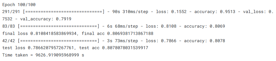
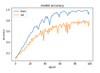
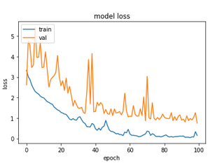
For the raw images dataset, our high ‘Patience’ value means that all the 100 epochs have been run, and yet the test accuracy obtained is considerably lower than had been accomplished by the cut-off ResNet50 (~81% instead of ~87%). The validation loss is much jumpier, and worst of all, though not unexpected, the run took almost 8 times longer. In short, there was no advantage to using the full ResNet at all on this dataset.

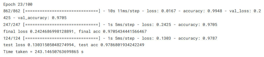
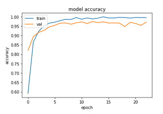
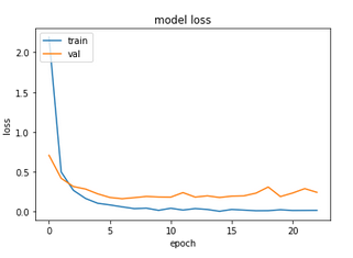
For the EMNIST-based dataset, we have:

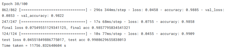
Here we at least see a reduction in the total number of epochs, although the time taken is again several times higher than even the 100 epochs that the cut-off ResNet had taken. This was the easiest dataset to fit the last time, and it’s no surprise that we again obtained almost a perfect accuracy.

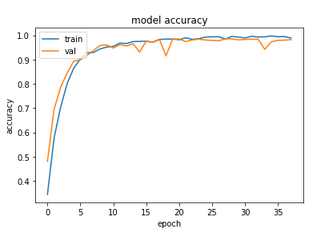
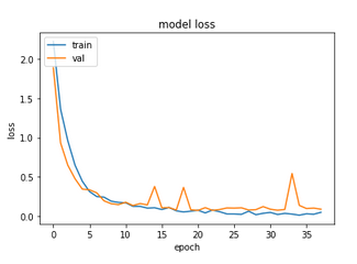
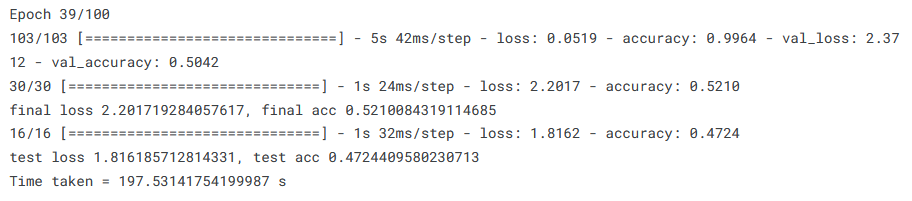
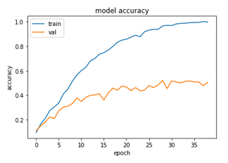
Finally we come to the Chars74K-based dataset:

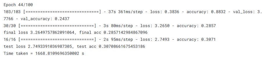
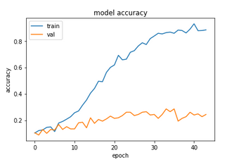
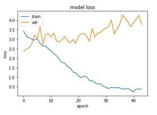
Arguably the worst results are obtained for this dataset, with test accuracy being half that obtained by the cut-off ResNet. The problem of overfitting seen last time has obviously been magnified by applying a bigger model.

We see that the results are different for the three datasets, but are rather discouraging overall. Now, we can undoubtedly improve the performance of the full ResNet - we have not applied any regularisation, BatchNormalization, Dropout, transfer learning weights, etc., etc. As a first pass, though, we can conclude that using the full ResNet50 on what are at the end of the day are fairly simple images is unlikely to lead to accuracy improvements that will be worth the added complexity and run times.

Simple CNN

What about a simpler network? Let us build a simple, no-frills CNN from scratch and see how it performs.

First the CNN itself is built as per the following code:

model_3 = tf.keras.models.Sequential([
    tf.keras.layers.Conv2D(16, (3,3), activation='relu', input_shape=(32, 32, 3)),
    tf.keras.layers.MaxPooling2D(2,2),
    tf.keras.layers.Conv2D(32, (3,3), activation='relu'),
    tf.keras.layers.MaxPooling2D(2,2),
    tf.keras.layers.Conv2D(64, (3,3), activation='relu'),
    tf.keras.layers.MaxPooling2D(2,2),
    tf.keras.layers.Flatten(),
    tf.keras.layers.Dense(512, activation='relu'),
    tf.keras.layers.Dense(10, activation='softmax')
])

Now for the results. For the raw images dataset we have:

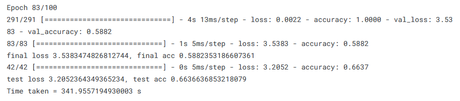
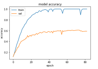
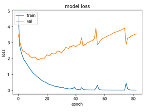
Well, the good news is that it was quick - only 342 s! The bad news is that the test accuracy is only 66%…

Let us see what the EMIST-dataset results are like:

If you have followed the previous runs on this dataset, you might have already guessed the results obtained - very quick run, and 98% test accuracy. Moving on to the Chars74K-dataset, we have:

In one sense, the results obtained are better than that which had been obtained for the cut-off ResNet - the validation loss curve is much smoother than what we saw last time. Although a good thing in itself, as too much fluctuation in the loss values is a sign of instability in training, ultimately it does not in this case lead to a higher, or even comparable, test accuracy, which is what really counts.

So we can conclude that the cut-off ResNet50 used by the competition organisers is in fact the best choice for this problem.

But wait, I hear some of you say - what about run time? Isn’t the simple CNN much faster than the cut-off ResNet? Well yes, but remember that we did not use early stopping for the cut-off ResNet. We can see what happens if we apply early stopping and run the cut-off ResNet on the Chars74K-based dataset - we get both lower run time (154 s against 198 s) and higher test accuracy (~53% against ~47%) for the cut-off ResNet. So the organisers certainly knew what they were doing when they selected this particular network!

Combined dataset

All right, so we are now ready for the final part of this particular journey. I mentioned earlier that we will be testing the best performing network on a combined dataset. Now that we have selected the winning network, let us see how it does on the final dataset.

The combined dataset I used contains all the files in the raw images and Chars-74k based datasets, along with 100 capital and 100 small letters for each number from the EMNIST-based dataset. The reason for using a limited number of EMNIST-based images is simple - using all the images (~10,000) would have led to this dataset providing the overwhelming majority of images in the combined dataset. As it now stands, the combined dataset is relatively well balanced, with almost 6,500 images split in a 70:20:10 training:validation:test set ratio. You can find this dataset here, while the evaluation code is here.

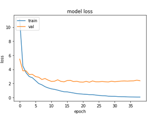
As per the usual procedure, let us see the accuracy values and the training curves:

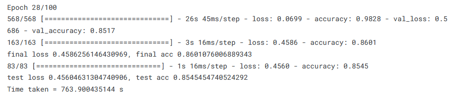
Not bad! We got a test accuracy of ~85%, while the training curves are also reasonably smooth, although some evidence of overfitting is present.

Data augmentation

Now, as the final touch, let us see if we can improve the results a little further by using image augmentation. Image augmentation is an easy way to generate subtly modified images on the fly, enhancing the number of images available for training. It also makes the model more robust against overfitting by teaching the model to recognise images despite changes such as distortions or orientation shifts. We will look at image augmentation in greater depth in the future, but for now let us just dip our toes.

The code used for the data augmentation is:

batch_size = 8

train_datagen = ImageDataGenerator(
        rotation_range=30,
        width_shift_range=0.1,
        height_shift_range=0.1,
        shear_range=0.1,
        zoom_range=0.1,
        fill_mode='nearest')

val_datagen = ImageDataGenerator()

test_datagen = ImageDataGenerator()

train = train_datagen.flow_from_directory(
        user_data,
        target_size=(32, 32),
        batch_size=batch_size)

valid = val_datagen.flow_from_directory(
        valid_data,
        target_size=(32, 32),
        batch_size=batch_size)

test = test_datagen.flow_from_directory(
        test_data,
        target_size=(32, 32),
        batch_size=batch_size)

You can read about the various parameters used in Keras’ ImageDataGenerator here. Although there are a large number of arguments that can be provided, I am only using rotation_range (the degrees by which the images can be rotated randomly), width_shift_range and height_shift_range (the fraction of the width and height by which to randomly move the images horizontally or vertically), shear_range (for random shear transformations) and zoom_range (for randomly zooming inside the images). Flipping, horizontally and/or vertically, is a commonly applied transformation, but a little thought will convince us that it is inappropriate here - a flipped ‘vii’ is no longer a 7…

It is important to remember that data augmentation, as a method to combat overfitting on the training set, is only applied to the training data, not the validation or test data. We therefore create two additional data generators for the validation and test sets without passing any arguments to these.

A brief point here - rescaling the images is generally recommended as an argument for all the data generators. By supplying ‘rescale = 1./255’, we ensure that the original 0-255 RGB pixel coefficients are reduced to a 0-1 range, which is more manageable for our models. In this case, however, rescaling led to noticeably worse results. This might be because the images are simple enough for the model to handle as-is, while rescaling led to information loss that impaired training. This is purely speculative, of course, and perhaps merits a more detailed look. For now, though, let us move forward without rescaling.

Once we have created the data generators, we need to feed them the appropriate data. As we are getting our data directly from the relevant directory, we can use Keras’ flow_from_directory for this purpose. As can be seen from the code above, all this means here is providing the folder name, the target image size, and the batch size.

Once the above code is run, we get the output:

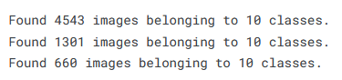
Perfect. We see that the training, validation and test images have been passed in, and the number of classes correctly detected from the number of folders (i-x) in each set.

Before running the model, let us have a look at the images. The code (rescaling is done here only to enable Matplotlib to plot the images, it has no effect on the modelling):

batch=next(train)
print([len(a) for a in batch])
# batch[0] are the images, batch[1] are the labels
# batch[0][0] is the first image,  batch[0][1] the next image

for i in range(len(batch[0])):
    img=(batch[0][i]/255)   
    fig = plt.figure()
    fig.set_size_inches(1,1)
    plt.imshow(img, aspect='auto')

And the output (random, so will differ from run-to-run):

For comparison, the validation images are:

We can see that the augmented training images are slightly harder to read, and have been rotated or moved up or down a little in some cases. We can certainly make the images more distorted, but ultimately, our aim is to make training a little harder for the neural network, not change the images so much that they bear little resemblance to the validation or test images.

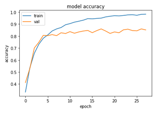
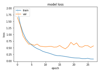
All right, so let us train our model the same way, and see the results:

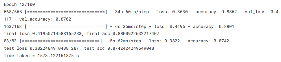
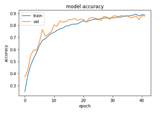
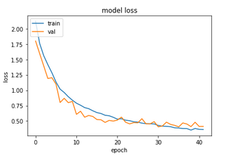
We see that the validation curve fluctuates more than earlier, but the overfitting appears to have been more or less eliminated. The test accuracy is now around 87.5% - not bad!

Is it possible to improve the accuracy further? Probably - for starters, we could look at hyperparameter optimisation to search for the ImageDataGenerator argument values that work best. We must be careful though - too much fine-tuning is a recipe for overfitting on the test set!

The above statement may confuse some. How can we overfit on the test set, when the model never sees it? Ah, the model doesn’t see it, but we do! We tinker with the parameters, run the model, and then look at the test accuracy. We then change the parameters some more, rerun the model, and see how the test accuracy was affected. At the end of it all, we feel that we have obtained the highest accuracy possible on the test set, which may be true, but we have ended up defeating the purpose of the test set, which is to provide a means to objectively assess the effectiveness of our model on unseen data. In other words, the test set is now simply a glorified extension to the training set. If tuned in this way, our model is unlikely to perform optimally on real unseen data.

Let us therefore be satisfied with what we have achieved - an accuracy in the late 80s on a fairly diverse and representative dataset, with a reasonable non-GPU run time of ~26 minutes. On to a new adventure next time!