4. Modelling water bodies - 1
Categories:
Tags:
Environment, Water, Kaggle, Competition
Hello again! The last few weeks, we have seen the creation and evaluation of handwritten Roman numerals datasets. This time, let us turn our attention to something different - the modelling of water levels in different water bodies.
One thing in common between this post and the previous ones is their origin in competitions I participated in. While the Roman numerals datasets were an output of my participation in the Data-Centric AI competition, the present post is based on my writeup for the Acea Smart Water Analytics competition organised on Kaggle from December 2020 - February 2021. Unlike the vast majority of Kaggle competitions, this particular competition was an ‘Analytics Competition’, which means that it had no leaderboard and no metric to fit to. Instead, competitors were asked to provide a notebook containing both, the models, and an explanation of the models. These notebooks were judged according to the criteria defined here - essentially, the soundness of the methodology, the quality of the presentation, and the applicability of the methods.
How did I do in this competition? Well, I at least made it to the list of finalists, which was something…then again, finishing in the top 17 out of 103 isn’t that great… In any case, in this series of posts, we will look at how I approached the problem. This post will describe the problem, why it matters, and the methodology I used, while the actual modelling and the results will be covered in future posts. The notebook containing all the code is available here, while the competition dataset is here. Please note that if you want to download the dataset, you will need to create a Kaggle account and accept the competition rules.
With that said, let’s go!
The problem
The competition was hosted by the Italian multiutility Acea SpA, which is involved in the water, energy and environmental sectors. As a water utility, one of the challenges they face is forecasting water body levels, which is important both in terms of ensuring water body health and adequately meeting water demand. This is made harder by the fact that they are in charge of different types of water bodies, with each type having unique characteristics, and so making generalisable models for predicting water levels is very difficult.
What the organisers wanted from the competitors therefore were four models that could be applied to one of the four categories of water bodies presented. A total of nine water bodies were present in the data - four aquifers, three water springs, one river and one lake. The aim was to determine how the particular features of a water body category influence the water availability. The organisers helpfully provided the following figure to explain what they were looking for:
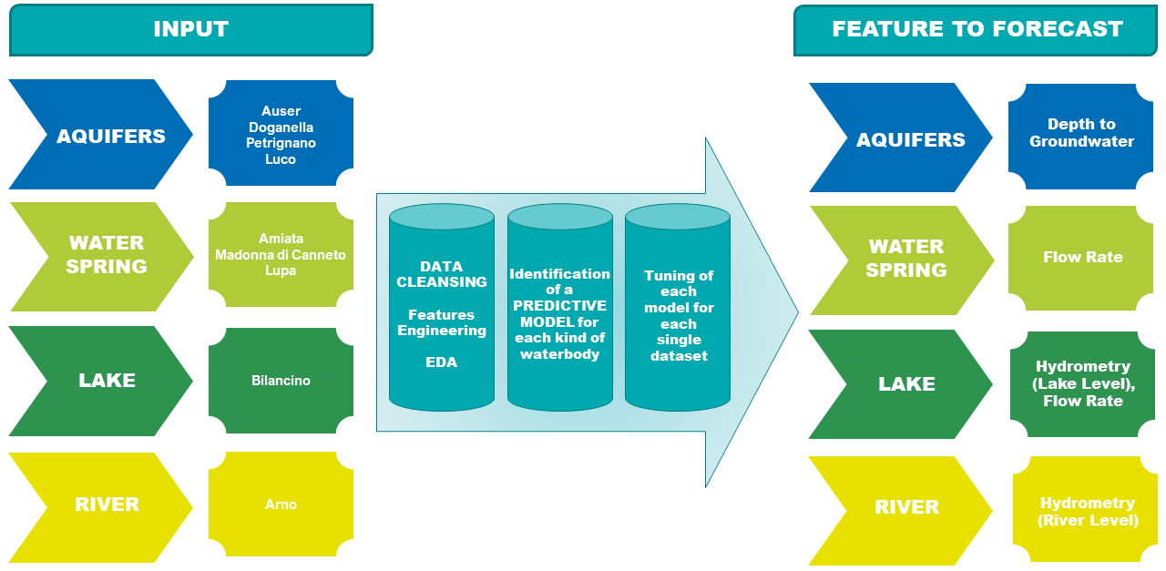
In reality, the modelling procedure follows a similar pattern for all the water bodies. We will look at that procedure next time - this post, as I said, will focus instead on the methodology used for the modelling.
Why it matters
Before heading into the methodological details, however, I think it might be worth explaining why I decided to enter this competition. Firstly, an analytics competition was appealing since it avoids my pet peeve about Kaggle competitions - a horde of competitors doing whatever it takes to get a 0.01% improvement on the target metric. I might rant on that some other time, but suffice to say that this competition allowed the rather unusual prospect of models being judged on their elegance and real-world applicability. The flip side, of course, was the inherent subjectivity of the evaluation, but then again, this is certainly the case in real life as well.
The second reason was that I felt the competition tackled a very important and somewhat underappreciated problem - water scarcity. We have all heard the phrase ‘water is life’, to the point that it has become something of a cliché. And yet, that statement hardly overstates the critical role played by water in our existence. Indeed, it is because water is so ubiquitous, something we all need and use on a daily basis, be it for drinking, bathing, cooking, cleaning, or watering our plants, that we take it for granted, neglecting to think of how we would fare in its absence.
Actually, the previous sentence is probably only applicable to a relatively privileged portion of the global population. While precise numbers are hard to calculate, as per some estimates, as many as four billion people may be said to be living under conditions of severe water scarcity, a situation that is likely to grow worse if present trends continue. Growing population, combined with an ever-increasing water footprint, means that water demand is likely to continue to rise till at least the middle of the century, which prompts the question - how will this demand be met?
Globally, the answer to this question thus far has usually been to simply overexploit water resources. The results of this approach are now plain to see in many parts of the world - disappearing lakes, drying rivers, depleted aquifers, dropping water tables… Climate change is unsurprisingly expected to make matters worse still. An aspect that is less appreciated, though, is how water scarcity itself begets further overexploitation of water. An example may be seen in California, USA, where a prolonged drought caused by over-damming of rivers caused a huge increase in groundwater pumping. Of course, groundwater depletion in turn causes a drop in river flows, creating a vicious cycle. This is in addition to the other adverse impacts of groundwater depletion, such as reduction in vegetation, land subsidence and saltwater intrusion.
I think the above paragraph, though depressing, has made its point - sustainable use of our water resources is no trifling matter, but ranks among the biggest challenges facing us today. While water conservation measures will no doubt have a huge role to play, proper management on the supply side is no less important. Another less obvious point from the above is that management of water resources is a complex subject not just because of the associated socio-economic considerations, but also because the dynamics of water extraction, replenishment, and the interplay between the various water resources is very complex. Consider an aquifer. The aquifer may be replenished by rainfall, but depending on the geology, there may be a time lag before its water levels rise due to the rain. The aquifer may feed or be fed by surface water sources like rivers or lakes - perhaps both. It may be connected to other underground aquifers, with the flows through this system determined by the levels of the components. The aquifer system may also change with time, due to environmental changes or other factors. This means that proper water resource management requires both an understanding of the factors affecting the resources and a model that can employ these factors to tell us how to optimally utilise the resources. In other words, it’s a problem that calls for interpretable machine learning.
Methodology
Based on the above, I decided to develop four interpretable machine learning models to forecast water levels for the nine different water bodies in the competition dataset. The guiding principles behind the model creation were simplicity, generalisability and robustness, while also attempting to predict as accurately as possible within these constraints.
The first thing to do when tackling any machine learning problem is to define the type of the problem. This problem was clearly an example of time series modelling - we were provided with features as a function of time, and asked to predict water volumes over a time interval (often multiple volumes, as we shall see next time). This brings us to the next question - what is the best approach to solve this problem?
Classical methods
The traditional solution for time series forecasting has been a group of ‘classical’ methods. These range from simple methods like autoregression and moving average to progressively more complicated methods like Seasonal Autoregressive Integrated Moving-Average with Exogenous Regressors (SARIMAX) and Vector Autoregression Moving-Average with Exogenous Regressors (VARMAX). These methods are time-tested, and despite recent hype about machine learning (ML), often still outperform ML methods on a range of data. Naturally then, I started out by trying to apply these methods to the competition dataset. After about a week, though, I decided that I needed to change tack, as the classical methods were simply not working well enough, or at all in some cases.
The first problem was trying to figure out which method to use. This choice needed to be made based on the number and types of the inputs and outputs. Consider the aquifers. The temperature and hydrometry data showed strong seasonal trends, implying that a SARIMA/SARIMAX type model should be considered. However, these models are univariate, meaning that they tackle a single input variable, and hence the interaction between the different variables is lost. A VAR/VARMAX type model solves this issue by considering multivariate inputs, but is most suitable for time series without trends or seasonal components. To an extent, this can be addressed by repeatedly differencing each time series till it is judged as stationary by a test like the Augmented Dickey Fuller Test (ADF Test) or KPSS test. Another concern is the way VAR-type models make their predictions. A VAR-type model works as follows: you feed in the data for all the series from, say, 2006-2021, and the model then issues a forecast based on this for all the series for 2022. What is desirable, though, is a model to which the values for the non-target items for 2022 can be supplied, with the model predicting the target items. That is to say, we provide the rainfall, humidity, temperature, etc. for 2022, and get the expected water flow as output. This needs the use of a different class of methods, which I will discuss later.
Leaving the above shortcomings aside, I found that the classical methods were less suitable for this task simply because their inherent shortcomings, nicely summed up here: to perform well, they require complete and ‘clean’ data, which was not the case here; they generally assume a linear relationship between the variables; they focus on a fixed temporal dependence, and on one-step forecasts. Rather than trying to patch over each of these shortcomings, I decided to see if there are alternative methods that are easier to use and more accurate, while also being sufficiently robust. This search brought me to two different ways of tackling the problem.
Neural networks
The term ‘neural networks’ has become so popular in recent years as to become almost synonymous with ‘artificial intelligence’. Quite simply, a neural network (NN) is a model that attempts to replicate the structure of the brain via a system of mathematical functions called ‘neurons’. These ‘neurons’ can be trained to learn the relationship between input information and the desired outputs, and a properly trained NN can then be deployed on unseen data. If fed sufficient training data, then large NNs, with dozens of layers and thousands of neurons, can significantly outperform traditional ML algorithms or statistical methods.
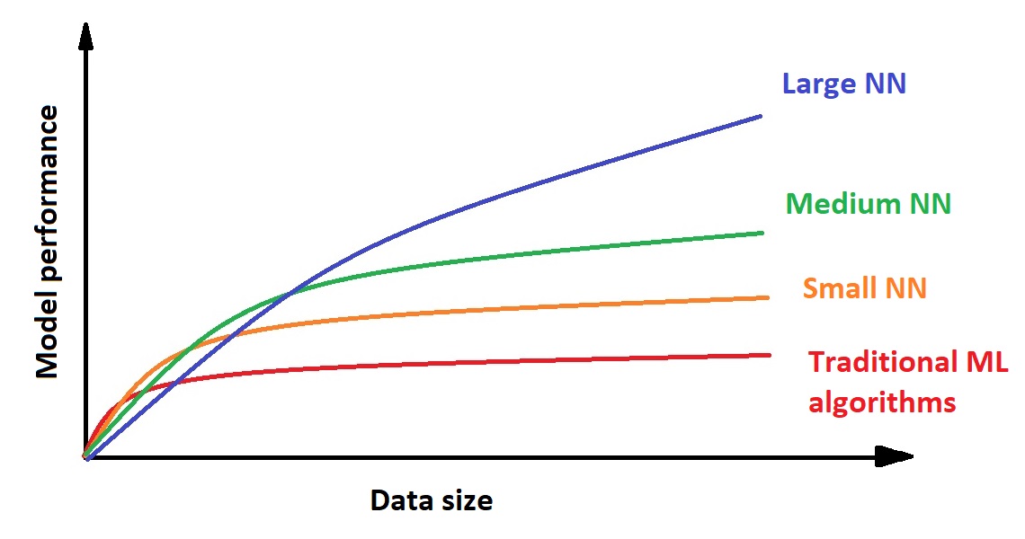
Advantage of neural networks (based on Andrew Ng’s talk available here)
The downside of NNs is that they require a large amount of data to outperform, and are computationally expensive. Anyway, among the different types of NNs, Recurrent Neural Networks (RNNs) are better suited to time series analysis, as their neurons contain a ‘memory state’ that helps them ‘remember’ the previous inputs and thus model sequential data. A traditional RNN, however, cannot model long-term dependencies in the data owing to the ‘vanishing gradient problem’ - simply put, it has a relatively short-term memory. Long-Short Term Memory networks (LSTMs) are specialised RNNs developed to tackle this issue, and these are therefore well-suited to time series modelling where long-term trends form an important part of the modelling inputs, as was the case here. A detailed explanation of these systems is beyond the scope of this post (later maybe…), and I refer you instead to the many excellent explanations found online (such as here, here or here). All that I will say here is that their robustness to noisy input data, ability to learn non-linear relationships in the data, and inherent support for multivariate, multi-step forecasts certainly make LSTMs worthy of further consideration for this competition dataset. At the same time, LSTMs need a large quantity of data to perform properly, which is not the case for several of the data series here. They also ideally require a large number of layers and training epochs, which is computationally unattractive. It is therefore pertinent to also look at another class of deep learning models.
Decision tree-based methods
A decision tree is an ML algorithm that takes decisions based on the responses to a series of yes or no questions about the data. A simple decision tree for predicting the possibility of the survival of passengers on the Titanic is shown below as an example.

Example of decision tree based on Titanic passengers data, taken from Wikimedia
While simple, a decision tree is not very useful by itself as a machine learning model, as it will overfit to the training data, and therefore be virtually useless for any new data. However, if numerous decision trees are trained on subsets of the data, the average of these predictions is much more accurate and robust than those of any single tree trained on the entire data. Two methods used for this are bagging and boosting. Random forest (RF) is a bagging method that is simple, easy to use, and resistant to overfitting, due to which it is one of the most widely used ML algorithms. On the flipside, making an accurate RF model requires lots of trees, and training these can be a slow process in the presence of large quantities of data. Boosting methods, if tuned properly, give better results than RFs. However, they are more sensitive to noisy data and require more careful tuning, as they are prone to overfitting.
With respect to the competition dataset, decision tree-based methods have some pros and cons. On the negative side, these methods have no awareness of time, as they assume that observations are independent and identically distributed. This limitation can be solved by feature engineering, particularly ‘time delay embedding’, in other words providing the model with time lags of the modelled data. Another concern is that these methods cannot extrapolate, i.e., predict values outside the range of the trained data. This can also be dealt with using feature engineering, such as differencing and statistical transforms, but for this competition, the predicted values are in any case unlikely to be outside the training data band, meaning that this disadvantage is not a major handicap.
While the above explains why decision tree-based methods can be used for time series modelling, it does not explain why they are a good option. The first reason they are a good option is that, unlike classical methods or LSTM, one can simply provide these models with the non-target item values and obtain the target predictions. This is useful since, at the end of the day, the aim of the exercise is to see how variables like rainfall and temperature influence the output variables like depth of groundwater. Secondly, it has been noted that interpretability is very important in making an effective model, and in this regard, decision tree-based methods are far superior to NN methods. As noted here, these methods help easily answer questions such as which inputs are the most important for the predictions, how they are related to the dependent variable and interact with each other, which particular features are most important for some particular observation, etc. Finally, the very fact that they work in a manner very different from NNs makes them useful in an ‘ensemble’.
Ensembling
I mentioned earlier that the reason a combination of the predictions of decision trees trained on subsets of the data outperforms that of a decision tree trained on the entire data is because their uncorrelated errors tend to cancel each other out. This is the basis of the ensembling principle, wherein several models making uncorrelated errors on different parts of the data can be combined to give a model with a much lower error rate and higher generalisability. Decion tree-based ensembles are an ensemble of ‘weak learners’, as the decision trees are not individually very good at making predictions. The ensembling principle can however be extended to ‘strong learners’, such as a combination of RFs and NNs. By offsetting each other’s weaknesses, they give more robust and accurate predictions, explaining why they are a staple of winning ML competition submissions. The added complexity is an undoubted disadvantage, and so it needs to be checked that the ensemble predictions are indeed better enough than those of the individual models to justify this extra complexity.
Models used
I performed some preliminary runs on the competition datasets, which showed that random forests, LightGBM (Light Gradient Boosting Machine, a decision tree boosting method) and long short-term memory neural networks were the best options, with each giving the best results for a certain portion of the data. I therefore decided to use these three methods, hereafter be referred to as RF, LGBM and LSTM. In addition, I also evaluated the results of an ensemble of these methods.
Metrics used
Before we can judge whether a model is ‘good’ or not, the metrics for determining the quality of the predictions need to first be fixed. Here, the competition organisers asked us to provide ‘a way of assessing the performance and accuracy of the solution’, in other words to provide a metric with justification. A range of error metrics are available, with Mean Absolute Error (MAE), Root Mean Square Error (RMSE), Mean Percentage Error (MPE), Mean Absolute Percentage Error (MAPE), Symmetric mean absolute percentage error (SMAPE), and Weighted Mean Absolute Percentage Error (WMAPE) among the proposed options for regression problems. Since all of these have shortcomings, and trying them all out was impractical, the first two options, which are the most widely used of the lot, were the only two I seriously considered. Unless there is a specific reason to penalise larger errors much more than smaller errors (i.e. an error of 10 is more than twice as bad as an error of 5), MAE is a better metric due to its better interpretability as compared to RMSE, which is actually a function of three different characteristics of errors, rather than of just the average error, making its interpretation ambiguous. However, regression algorithms such as sklearn’s RandomForestRegressor tend to be far slower if MAE is used as a splitting criterion rather than RMSE. This was not a handicap, though - I was interested in using MAE as a model evaluation criterion, so the split criterion used in the algorithm is irrelevant. In other words, the RMSE was used earlier in the modelling process to train the model, and then the performance of the model was later determined using MAE. I anyway provided the RMSE of all the models as well, but only as a reference, not for deciding model performance.
Model interpretation
I have already stated that model interpretability is very important in ML, and that decision tree ensembles are superior in this regard to NNs. For RFs, for example, the decision on how to split a tree is based on an ‘impurity’ measure like Gini impurity, and the Mean Decrease Impurity (MDI) can be itself be used as a gauge of feature importance. MDI, however, tends to inflate the importance of continuous or high cardinality variables compared to lower cardinality categorical variables, meaning that a variable than has a 1000 levels is likely to be ranked higher than one with 3 levels regardless of the actual contribution to the target prediction. Besides, as the MDI is calculated on the training set, it can give high importances to variables that are not actually predictive of the target but which could potentially be used to overfit. The solution is to use permutation importance - further details can be found here and here.
While permutation importance can be and has been used here for the tree-based methods, the LSTM is a ‘black box model’, and therefore requires a different interpretation mechanism. Several interpretation methods have been proposed in recent years, of which SHAP (SHapely Additive exPlanations) and LIME (Local Interpretable Model-agnostic Explanations) are perhaps the two most prominent (see here and here for detailed explanations). While neither is perfect, the main advantage of LIME appears to be speed, while SHAP appears to be a better overall choice for model interpretation, especially if one is trying to explain the entire model rather than a single prediction. While I initially tried using both simultaneously, this became unwieldy and hard to work with when applied to all the models, and hence decided to stick with SHAP, which I applied to all the models, including the tree-based ones. The details of the SHAP mechanisms can be better understood when we look at the actual runs, and will therefore be provided there.
Conclusion
OK, so this was a text-heavy post where I covered the methodology in plenty of depth. I think, though, that this detailed background was necessary to understand why I made the modelling choices I did. With that out of the way, next time we will see the actual modelling of the water bodies. So long!