5. Modelling water bodies - 2
Categories:
Tags:
Environment, Water, Pandas, Kaggle, Competition, Imputation, Matplotlib
[Edit: This and the next post were originally published as one, but I have now split them to improve readability.]
Welcome back. The last time we saw the details of the methodology that I used to tackle the Acea Smart Water Analytics competition. Now, let’s see the actual modelling of the water bodies. While the notebook containing all the code (available here) deals with all the waterbodies, the procedure is repetitive, and so we will look in detail in this post at only one representative water body. As you will see, there’s plenty to unpack for that one!
Before we start, the competition’s data page helpfully points out one of the challenges involved in the modelling:
It is of the utmost importance to notice that some features like rainfall and temperature, which are present in each dataset, don’t go alongside the date. Indeed, both rainfall and temperature affect features like level, flow, depth to groundwater and hydrometry some time after it fell down. This means, for instance, that rain fell on 1st January doesn’t affect the mentioned features right the same day but some time later. As we don’t know how many days/weeks/months later rainfall affects these features, this is another aspect to keep into consideration when analyzing the dataset.
OK, keeping that in mind, let us get to the modelling. This post will deal with the data wrangling/munging aspects, with the actual modelling handled next time.
Aquifer Petrignano
The water body I have selected to demonstrate the modelling here is Aquifer Petrignano, one of the four aquifers present in the dataset. As per the stated goal of the competition, this ‘aquifer’ model I built is applicable to each aquifer. Only the initial data wrangling portion requires some manual intervention, while the rest of the process is automated and identical for each aquifer.
The competition data page describes the Petrignano aquifer as follows:
The wells field of the alluvial plain between Ospedalicchio di Bastia Umbra and Petrignano is fed by three underground aquifers separated by low permeability septa. The aquifer can be considered a water table groundwater and is also fed by the Chiascio river. The groundwater levels are influenced by the following parameters: rainfall, depth to groundwater, temperatures and drainage volumes, level of the Chiascio river.
The reason I chose this aquifer to demonstrate is since it has all the column types associated with aquifers (rainfall, depth to groundwater, temperature, volume and hydrometry), and only two target variables, unlike some of the other water bodies. The methods for loading and visualising the data, filling in the missing values, and the various modelling steps are largely similar for all the water bodies, and so I will take the time to explain these in detail.
Data loading and visualisation
The first thing to do is to load the dataset. For every water body I loaded the csv file in an identical fashion, to keep things general. As is customary for dealing with tabular data in Python, the pandas library has been used for all the data loading.
# Load the dataset
train = pd.read_csv('../input/acea-water-prediction/Aquifer_Petrignano.csv', parse_dates=['Date'], dayfirst=True)
# Create a copy of the original data, since the 'train' dataframe will be modified
train_orig = train.copy()
Let us now look at the start and end of the data, as well as the columns in the dataframe.
train.head()
train.tail()
train.info()| Date | Rainfall_Bastia_Umbra | Depth_to_Groundwater_P24 | Depth_to_Groundwater_P25 | Temperature_Bastia_Umbra | Temperature_Petrignano | Volume_C10_Petrignano | Hydrometry_Fiume_Chiascio_Petrignano | |
|---|---|---|---|---|---|---|---|---|
| 0 | 2006-03-14 | NaN | -22.48 | -22.18 | NaN | NaN | NaN | NaN |
| 1 | 2006-03-15 | NaN | -22.38 | -22.14 | NaN | NaN | NaN | NaN |
| 2 | 2006-03-16 | NaN | -22.25 | -22.04 | NaN | NaN | NaN | NaN |
| 3 | 2006-03-17 | NaN | -22.38 | -22.04 | NaN | NaN | NaN | NaN |
| 4 | 2006-03-18 | NaN | -22.60 | -22.04 | NaN | NaN | NaN | NaN |
| Date | Rainfall_Bastia_Umbra | Depth_to_Groundwater_P24 | Depth_to_Groundwater_P25 | Temperature_Bastia_Umbra | Temperature_Petrignano | Volume_C10_Petrignano | Hydrometry_Fiume_Chiascio_Petrignano | |
|---|---|---|---|---|---|---|---|---|
| 5218 | 2020-06-26 | 0.0 | -25.68 | -25.07 | 25.7 | 24.5 | -29930.688 | 2.5 |
| 5219 | 2020-06-27 | 0.0 | -25.80 | -25.11 | 26.2 | 25.0 | -31332.960 | 2.4 |
| 5220 | 2020-06-28 | 0.0 | -25.80 | -25.19 | 26.9 | 25.7 | -32120.928 | 2.4 |
| 5221 | 2020-06-29 | 0.0 | -25.78 | -25.18 | 26.9 | 26.0 | -30602.880 | 2.4 |
| 5222 | 2020-06-30 | 0.0 | -25.91 | -25.25 | 27.3 | 26.5 | -31878.144 | 2.4 |
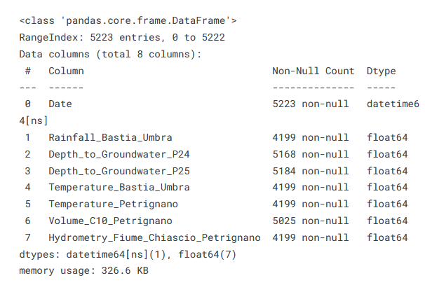
We see that the data starts in March 2006 and ends in June 2020, and that there are 7 columns in all: 1 Date, 1 Rainfall, 2 Depth to Groundwater, 2 Temperature, 1 Volume and 1 Hydrometry. We also see that there are lots of missing values, especially at the start of the data - the Date column, which has an entry for each row, has 5223 non-null values, while some of the columns have only 4199. It is clear that missing value imputation will play a key part - we will discuss that in detail later. Before that though, let us make a list of the target columns - a step that obviously must be done manually.
targets = ['Depth_to_Groundwater_P24', 'Depth_to_Groundwater_P25']
Next, I decided to remove all the February 29 rows from the data, since otherwise there are issues later on in the modelling process, all years other than leap years having 365 days. Since a leap day only occurs once every 1461 days, there is minimal loss of data. The following cell removes the leap days via masking.
def is_leap_and_29Feb(s):
    return (s.Date.dt.year % 4 == 0) & \
           ((s.Date.dt.year % 100 != 0) | (s.Date.dt.year % 400 == 0)) & \
           (s.Date.dt.month == 2) & (s.Date.dt.day == 29)

mask = is_leap_and_29Feb(train)

train = train.loc[~mask]
OK, the next step is removing those rows at the start of the dataframe that do not have values for one or more of the target variables. Why is this needed? While it is not the case for Aquifer Petrignano, there are some datasets where target values are not available for several years at the beginning. Imputing values and using these rows for model training is incorrect, as the model will learn to predict the imputed data instead of fulfilling the aim of matching the actual data. I therefore wrote the cell below to find out the maximum length of NaNs before a valid value for any of the target columns, and remove all the dataframe rows before this value. Any missing values in the targets that occur later in the dataframe will be imputed. Doesn’t this contradict what I just said about imputation being inappropriate? Well, the gaps in data in the middle are a lot less numerous than the large gaps in the beginning, and so imputing these is an acceptable trade-off here.
i = 0
nan_len = []
while i<len(targets):
    nan_len.append(train[f'{targets[i]}'].notna().idxmax())
    i += 1

train = train.iloc[max(nan_len):].reset_index(drop = True)
Let us now see how the data looks visually, which will help determine if any data wrangling other than missing value imputation is needed. I should note here that I used a light touch to data wrangling, only making any changes to the data where I felt it was both necessary and justified.
The cell below creates separate dataframes for each type of variable (e.g. rainfall, volume, etc.), both for ease of plotting and because they come in handy later in the modelling process. A list of the columns corresponding to that variable type is also created for later use.
rain_df = train.filter(regex=("Rainfall.*"))
rains = rain_df.columns.tolist()
rain_df.insert(0, column = 'Date', value = train['Date'])

vol_df = train.filter(regex=("Volume.*"))
vols = vol_df.columns.tolist()
vol_df.insert(0, column = 'Date', value = train['Date'])

temp_df = train.filter(regex=("Temperature.*"))
temps = temp_df.columns.tolist()
temp_df.insert(0, column = 'Date', value = train['Date'])

depth_df = train.filter(regex=("Depth_to_Groundwater.*"))
depths = depth_df.columns.tolist()
depth_df.insert(0, column = 'Date', value = train['Date'])

hydro_df = train.filter(regex=("Hydrometry.*"))
hydros = hydro_df.columns.tolist()
hydro_df.insert(0, column = 'Date', value = train['Date'])
Now let us plot the different variables (using Matplotlib, as ever). You will notice that all the plot codes are contained inside a if statement that checks if the particular type of variable exists. If, for instance, there is no hydrometry term, the length of the hydrometry list created earlier will be 0, and the code will not run. This takes care of different datasets not having all the different variable types (a recurrent problem), ensuring that the model runs smoothly and automatically for every dataset.
First, the rainfall:
if len(rains)>0:
    i = 0
    while i<len(rains):
        if i == 0:
            ax1 = rain_df.plot.scatter(x = 'Date', y = f'{rains[i]}', color=colours[i])
        else:
            axes = rain_df.plot.scatter(x = 'Date', y = f'{rains[i]}', color=colours[i], ax = ax1)
        y_axis = ax1.yaxis
        y_axis.set_label_text('Rainfall (mm)')
        i += 1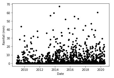
We can see that for the rainfall, the graph is as expected. Most of the days receive no rainfall, the average rainy day sees perhaps 10-20 mm of rain, while there are a few exceptional days that have values greater than 50 mm. Note the X-axis; the rainfall data is only available from 2009.
Next, the ‘volume’:
if len(vols)>0:
    i = 0
    while i<len(vols):
        if i == 0:
            ax1 = vol_df.plot.scatter(x = 'Date', y = f'{vols[i]}', color=colours[i])
        else:
            axes = vol_df.plot.scatter(x = 'Date', y = f'{vols[i]}', color=colours[i], ax = ax1)
        y_axis = ax1.yaxis
        y_axis.set_label_text('Volume (m$^3$)')
        i += 1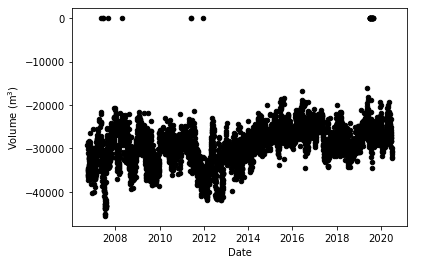
The volume term refers to the amount of water taken from the drinking water treatment plant, a critical parameter in determining its health. Here, we see that most of the days had water extraction of roughly 30000 m3, with no clear trends visible.
if len(temps)>0:
    i = 0
    while i<len(temps):
        if i == 0:
            ax1 = temp_df.plot.scatter(x = 'Date', y = f'{temps[i]}', color=colours[i])
        else:
            axes = temp_df.plot.scatter(x = 'Date', y = f'{temps[i]}', color=colours[i], ax = ax1)
        y_axis = ax1.yaxis
        y_axis.set_label_text('Temperature ($^o$C)')
        i += 1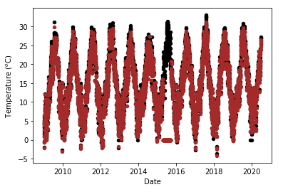
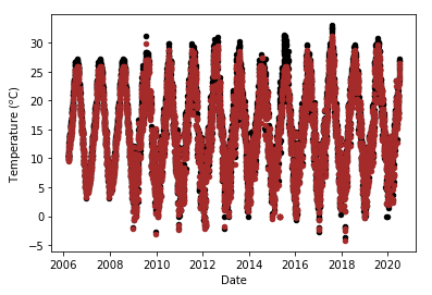
The two temperature terms show a seasonal trend, with maximum temperatures of around 30 oC towards the middle of the year, and a minimum value of around 0 oC around the turn of the year. This is as expected; after all seasons are virtually defined by the rise and fall in temperatures. This seasonality will be used for imputing missing temperature data.
if len(depths)>0:
    i = 0
    while i<len(depths):
        if i == 0:
            ax1 = depth_df.plot.scatter(x = 'Date', y = f'{depths[i]}', color=colours[i])
        else:
            axes = depth_df.plot.scatter(x = 'Date', y = f'{depths[i]}', color=colours[i], ax = ax1)
        y_axis = ax1.yaxis
        y_axis.set_label_text('Depth to groundwater (m)')
        i += 1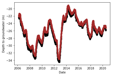
‘Depth to groundwater’ refers to the groundwater level measured in terms of distance from the ground floor as detected by a piezometer. As the target variables for aquifers are the depth to groundwater terms, this is obviously a very important variable category. The two depth to groundwater terms in this dataset follow each other very closely, and both show a highly haphazard pattern, with the values dropping and rising by large amounts at seemingly random intervals.
if len(hydros)>0:
    i = 0
    while i<len(hydros):
        if i == 0:
            ax1 = hydro_df.plot.scatter(x = 'Date', y = f'{hydros[i]}', color=colours[i])
        else:
            axes = hydro_df.plot.scatter(x = 'Date', y = f'{hydros[i]}', color=colours[i], ax = ax1)
        y_axis = ax1.yaxis
        y_axis.set_label_text('Hydrometry (m)')
        i += 1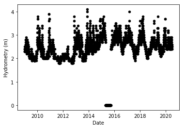
Finally, we come to the hydrometry term, which is also a measure of the groundwater level, but as determined by a hydrometric station rather than using a piezometer. We see from the figure that this variable is more stable than the depth to groundwater terms, and it exhibits a mild seasonal pattern, far less pronounced than for temperatures.
Data imputation
As I said earlier, data imputation plays a major part in tackling this competition dataset. Different imputation methods are suitable for the different variable types, as will be seen below. An additional point is that the imputation should occur not just for missing values, but also to replace erroneous data, if these can be definitively identified.
Let us start with rainfall. For rainfalls, since 0 is a legitimate value, and is in fact the mode of the data, and since there is no theoretical upper limit to the amount of rain received, the only way any data can be identified as wrong is in the case of negative values or values perhaps a hundred times greater than the rest. This is not the case for any of the datasets, and hence we can focus simply on imputing the missing data. Using the monthly average of the rainfall may be one possible method, but as we saw in the rainfall graph above, there is no seasonality in the data, and hence using monthly averages to impute long stretches of time will probably bias the data. As per the KISS principle, complexity should be avoided unless necessary. In the case of rainfall, inserting the mode value of 0 (i.e. no rainfall on that day) in place of the missing data is the simplest solution, and in the absence of any better alternatives, I decided to use this.
if len(rains)>0:
    i = 0
    while i<len(rains):
        train[f'{rains[i]}'] = train[f'{rains[i]}'].fillna(0)
        i += 1
Next, the volume. As mentioned above, the volume term refers to the amount of water taken from the drinking water treatment plant. It can therefore have a value of 0 if no water is taken on that day. The same points as made for rainfall also hold for volume, and therefore I did the imputation the same way too.
if len(vols)>0:
    i = 0
    while i<len(vols):
        train[f'{vols[i]}'] = train[f'{vols[i]}'].fillna(0)
        i += 1
We have seen that the temperature terms show a seasonal trend as expected, and I used this for imputation. The invalid data is a little hard to identify here, given that the data correctly has positive, negative and zero values. Again, values far outside the range of the rest of the data may be erroneous, and a statistical measure like the z-score may be used to identify these outliers. An inspection of the minimum and maximum values of the temperature data for all the datasets did not turn up anything untoward, and hence I decided to skip further statistical inspection. Another source of erroneous data, however, does appear to exist - long stretches of time with values of 0, likely indicating corrupt data. Somewhat arbitrarily, I decided that 7 or more consecutive values of 0 were errors, and decided to mask and replace these with NaNs for imputation.
if len(temps)>0:
    i = 0
    while i<len(temps):
        a = train[f'{temps[i]}'] == 0
        mask = a.cumsum()-a.cumsum().where(~a).ffill().fillna(0) >= 7
        train[f'{temps[i]}'] = train[f'{temps[i]}'].mask(mask, np.nan)
        temp_df[f'{temps[i]}'] = temp_df[f'{temps[i]}'].mask(mask, np.nan)
        i += 1

# Replacing 7 or more 0 temperature values with Nans
# Taken from
#https://stackoverflow.com/questions/42946226/replacing-more-than-n-consecutive-values-in-pandas-dataframe-column
That done, we can now turn to the actual data imputation, which is done in the cell below.
if len(temps)>0:
    i = 0
    while i<len(temps):
        X = pd.DataFrame(temp_df.iloc[:, np.r_[0,i+1]])
        X['dayofyear'] = X['Date'].dt.dayofyear
        X2 = X.groupby('dayofyear').mean()
        X2.reset_index(level=0, inplace=True)
        X.loc[X[f'{temps[i]}'].isnull() == True, 'same_day'] =\
        X['dayofyear'].map(X2.set_index('dayofyear')[f'{temps[i]}'].to_dict())
        X.loc[X[f'{temps[i]}'].isnull() == False, 'same_day'] = X[f'{temps[i]}']
        X.loc[X[f'{temps[i]}'].isnull() == True, f'{temps[i]}' + '_new'] = X['same_day']
        X.loc[X[f'{temps[i]}'].isnull() == False, f'{temps[i]}' + '_new'] = X[f'{temps[i]}']

        train[f'{temps[i]}'].update(X[f'{temps[i]}' + '_new'])

        i += 1

    i = 0
    while i<len(temps):
        if i == 0:
            ax1 = train.plot.scatter(x = 'Date', y = f'{temps[i]}', color=colours[i])
        else:
            axes = train.plot.scatter(x = 'Date', y = f'{temps[i]}', color=colours[i], ax = ax1)
        y_axis = ax1.yaxis
        y_axis.set_label_text('Temperature ($^o$C)')
        i += 1
Briefly, the average temperature for each day of the year is calculated, and this average is used to fill in missing data for that date. For example, if the temperature value for June 29, 2018 is missing, then the average temperature of June 29 calculated using the rest of the data will be filled in. As we can see from the figures showing the original (left) and the imputed data (right) below, this method works very well. In the original temperature data, you see that the ‘red’ graph has a big stretch of zeroes around 2015, and the updated graph looks much more reasonable in this timespan.
Next, let us turn to the hydrometry term, which also has a weak seasonal pattern, and hence can be imputed similarly to temperature. Unlike all the previous items, however, the 0 values here can be considered as errors - the values cannot suddenly depart from their usual 2-4 m range and become 0. Therefore, I replaced all the 0 values by NaNs. I made a fresh dataframe for the hydro terms from the imputed data, for reasons that I will explain when I touch upon Aquifer Auser. The rest of the procedure is the same as for temperature. The figure below shows that this imputation method gives adequate results for hydrometry, though less realistic than was the case for temperature.
if len(hydros)>0:
    i = 0
    while i<len(hydros):
        train[f'{hydros[i]}'].replace(0, np.nan, inplace=True)
        i += 1
# 0s in hydros are errors, so replace them with Nans
    hydro_df2 = train.filter(regex=("Hydrometry.*"))
    hydros = hydro_df2.columns.tolist()
    hydro_df2.insert(0, column = 'Date', value = train['Date'])

That leaves only one more term to deal with. I have kept the depth of groundwater term for the last, since this is easily the most difficult to impute. Going over all the different datasets, no one method, e.g. mean, rolling mean, fill forward, K-nearest neighbours, seasonal interpolation, etc. worked well for every depth of groundwater series. This left me with two alternatives - either use a bespoke imputation method for each depth of groundwater after manual inspection and analysis, or use a multiple imputation method. Multiple imputation methods compensate for the uncertainty in the missing data by creating and combining predictions from several plausible imputed datasets. Their use permits automatic processing, which was one of my aims, and hence I decided to use these for imputing the depth of groundwater data. The question, though, was: which of the several different multiple imputation methods should I use?
Again, there is no perfect solution, but some studies/opinions show that the RF-based MissForest algorithm (details can be found here or here) can outperform alternatives like MICE and Hmisc. We will therefore use this method. The original MissForest algorithm was implemented in R, and sklearns’ IterativeImputer, which has an ExtraTreesRegressor estimator similar to MissForest is currently experimental and not stable. I therefore used the missingpy module. I carried out the imputation on a copy of the original dataset to avoid the fitting being influenced by the imputations of the other variables carried out above. Like with the hydrometry term, I treated 0 values as missing data. As the algorithm cannot handle ‘Date’ terms, and they are not necessary for the imputation anyway, I dropped the Date column prior to the run, and then added it back to the imputed dataframe.
imputer = MissForest()
train_copy = train_orig.copy()
if len(depths)>0:
    i = 0
    while i<len(depths):
        train_copy[f'{depths[i]}'].replace(0, np.nan, inplace=True)
        i += 1
# 0s in depths are errors, so replace them with Nans
    train_copy = train_copy.drop(['Date'], axis=1)
    col_list = list(train_copy)
    imputs = imputer.fit_transform(train_copy)
    imputs = pd.DataFrame(data=imputs, columns=col_list)
    imputs['Date']= train_orig['Date']
The imputed values are used to replace the missing values in the cell below:
if len(depths)>0:
    i = 0
    while i<len(depths):
        X = pd.DataFrame(depth_df.iloc[:, np.r_[0,i+1]])
        X.loc[X[f'{depths[i]}'].isnull() == True, f'{depths[i]}' + '_new'] =\
        X['Date'].map(imputs.set_index('Date')[f'{depths[i]}'].to_dict())
        X.loc[X[f'{depths[i]}'].isnull() == False, f'{depths[i]}' + '_new'] = X[f'{depths[i]}']
        train[f'{depths[i]}'] = X[f'{depths[i]}' + '_new']
        i += 1
    i = 0
    while i<len(depths):
        if i == 0:
            ax1 = train.plot.scatter(x = 'Date', y = f'{depths[i]}', color=colours[i])
        else:
            axes = train.plot.scatter(x = 'Date', y = f'{depths[i]}', color=colours[i], ax = ax1)
        y_axis = ax1.yaxis
        y_axis.set_label_text('Depth to groundwater (m)')
        i += 1
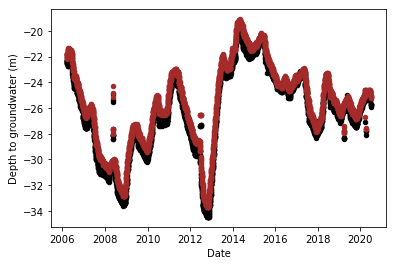
It must be said that the plot showing the imputed data (below, right) is not the best advertisement for MissForest, as there are some fitted points above and below the actual values. Overall, though, I found MissForest to be the most reliable and generalisable of all the imputation methods I tried on all the different depth of groundwater series, and hence decided to stick with it.
Forecast period
After concluding the data inspection and imputation, we are finally ready to look at the actual models. The first thing I had to decide is the time frame for which we want the predictions, i.e. how many days ahead do we want to predict. There was plenty of discussion on this topic in the competition forums, and it was stated by the organisers that the prediction period is difficult to predetermine, but needs to be decided on a case-by-case basis depending on the water body type and other factors. I therefore created a variable called days_ahead that allows the user to specify the desired time period, the model automatically forecasting for that period. The default value I used is 7 days, but I also ran it for 30 days for this waterbody to show how it works and how the predictions are affected by the forecast period.
days_ahead = 7

target_cols = targets.copy()
i = 0
for target in targets:
    train[target + '_target'] = train[target].shift(-days_ahead)
    target_cols[i] = target + '_target'
    i += 1
# Creating new columns by shifting the target columns by the forecast period
train = train.dropna()
# Required as the shift in the cell above introduces some new NaNs
Conclusion
All the initial groundwork is finished now, and the actual modelling can be done. As this post is long enough already, we will look at the three different types of models I used in the next post. So long!