Modelling water bodies - 3 | Agneev’s DS/ML lab book

Categories:

Data Science Machine Learning Python Time series Tabular

Tags:

Environment, Water, Pandas, Kaggle, Competition, Random Forest, LightGBM, LSTM, SHAP, Matplotlib, Ensemble

[Edit: This and the previous post were originally published as one, but I have now split them to improve readability.]

Hello! The last time we looked at the data wrangling aspects on data for Aquifer Petrignano in the Acea Smart Water Analytics competition. Now, let’s tackle the modelling. As a reminder, the complete code is available on Github, but we will only look at the main bits here. First, let’s look at a Random Forest (RF) model.

Random forest model

Before anything else, we should make a copy of the train dataframe that we have carried out all the data wrangling on, since that dataframe will also be used for the LGBM and LSTM models. The next thing is to carry out the feature engineering needed for a tree-based model to make predictions. This involves calculating the rolling mean for the variables where the cumulative sum is meaningful for modelling (i.e. rainfall and volume - the sum of the daily rainfall over a week can be an important input to the model) and the lag terms where this sum is meaningless (i.e. temperatures, hydrometry and depth of gorundwater - the ‘sum’ of the daily temperature over a week has no utility as such). Based on preliminary tests, separate rolling mean terms for every 30 days till 180 days and four lag terms till 90 days work sufficiently well without being either an excessive or an insufficient number of terms, and hence these are calculated in the cell below.

train_rf = train.copy()

if len(rains)>0:
    for r in rains:
        train_rf[r + '_roll_030'] = train_rf[r].rolling(30).mean().astype('float32')
        train_rf[r + '_roll_060'] = train_rf[r].rolling(60).mean().astype('float32')
        train_rf[r + '_roll_090'] = train_rf[r].rolling(90).mean().astype('float32')
        train_rf[r + '_roll_120'] = train_rf[r].rolling(120).mean().astype('float32')
        train_rf[r + '_roll_150'] = train_rf[r].rolling(150).mean().astype('float32')
        train_rf[r + '_roll_180'] = train_rf[r].rolling(180).mean().astype('float32')
if len(vols)>0:
    for v in vols:
        train_rf[v + '_roll_030'] = train_rf[v].rolling(30).mean().astype('float32')
        train_rf[v + '_roll_060'] = train_rf[v].rolling(60).mean().astype('float32')
        train_rf[v + '_roll_090'] = train_rf[v].rolling(90).mean().astype('float32')
        train_rf[v + '_roll_120'] = train_rf[v].rolling(120).mean().astype('float32')
        train_rf[v + '_roll_150'] = train_rf[v].rolling(150).mean().astype('float32')
        train_rf[v + '_roll_180'] = train_rf[v].rolling(180).mean().astype('float32')
if len(temps)>0:
    for t in temps:
        train_rf[t + '_week_lag'] = train_rf[t].shift(7).astype('float32')
        train_rf[t + '_month_lag'] = train_rf[t].shift(30).astype('float32')
        train_rf[t + '_bimonth_lag'] = train_rf[t].shift(60).astype('float32')
        train_rf[t + '_quarter_lag'] = train_rf[t].shift(90).astype('float32')
if len(hydros)>0:
    for h in hydros:
        train_rf[h + '_week_lag'] = train_rf[h].shift(7).astype('float32')
        train_rf[h + '_month_lag'] = train_rf[h].shift(30).astype('float32')
        train_rf[h + '_bimonth_lag'] = train_rf[h].shift(60).astype('float32')
        train_rf[h + '_quarter_lag'] = train_rf[h].shift(90).astype('float32')
if len(depths)>0:
    for d in depths:
        train_rf[d + '_week_lag'] = train_rf[d].shift(7).astype('float32')
        train_rf[d + '_month_lag'] = train_rf[d].shift(30).astype('float32')
        train_rf[d + '_bimonth_lag'] = train_rf[d].shift(60).astype('float32')
        train_rf[d + '_quarter_lag'] = train_rf[d].shift(90).astype('float32')

If the non-shifted target terms are kept in the dataframe, then the RF focusses on using those to predict the shifted target terms, which is contrary to our aim of getting it to predict based on the input variables. These are therefore dropped in the next cell. Alongside, the lag terms introduce NaNs at the start of the dataframe which will also be removed in the following cell in the same way we saw last time. The dropna removes all rows containing NaN, and the index[0] gives the first row of the resulting dataframe.

i = 0
for target in targets:
    train_rf = train_rf.drop([f'{targets[i]}'], axis=1)
    i +=1
# If the target columns are not removed, the RF just focuses on them.
train_rf = train_rf.loc[train_rf.dropna().index[0]:].reset_index(drop = True)

Now we are ready to split the dataframe into the train and test sets. Since we are trying to see how good our model is at predicting the future, the final year of data, i.e. from 1/7/2019 to 30/6/2020 will be used as the test set, with all the earlier data being used for training. We will further split the data into X (input) and y (output) terms. All this is done in the following cell.

rf_X = train_rf[train_rf.columns.difference(target_cols)]
rf_y = train_rf[target_cols]
train_rf_X = rf_X.iloc[:rf_X.loc[rf_X['Date'] == '2019-07-01'].index.item()].reset_index(drop = True)
test_rf_X = rf_X.iloc[rf_X.loc[rf_X['Date'] == '2019-07-01'].index.item():].reset_index(drop = True)
train_rf_y = rf_y.iloc[:rf_y.loc[rf_X['Date'] == '2019-07-01'].index.item()].reset_index(drop = True)
test_rf_y = rf_y.iloc[rf_y.loc[rf_X['Date'] == '2019-07-01'].index.item():].reset_index(drop = True)
# Note that rf_y does not have a Date column, but as it's the same length as rf_X,
# the Date column from that df can be used for the train-test split
col_list2 = list(train_rf.columns)
train_rf_X = train_rf_X.drop(['Date'], axis=1)
test_rf_X = test_rf_X.drop(['Date'], axis=1)
# The Date column needs to be removed for the RF regressor to work

Now, I want to clarify one thing to prevent any misgivings on the issue. The rolling and lag terms for the first few items of the test set will be based on data from the end of the training set. Is this data leakage? No.

Data leakage refers to ‘when the data you are using to train a machine learning algorithm happens to have the information you are trying to predict’. This is not the case here, as we are not trying to predict any of the rolling or lag terms. Further, we can see in the above link that leakage occurs due to ‘leaking data from the test set into the training set’, ‘leaking the correct prediction or ground truth into the test data’, ‘leaking of information from the future into the past’ and ‘information from data samples outside of scope of the algorithm’s intended use’. None of these is the case here.

In short, leakage only occurs if information that will not be available at prediction time is used in model training. All the lag and rolling means terms are in the past and thus will be available at prediction time, and hence this is not a data leak.

Having clarified the above point, we can now run the RF regressor. I maintained the default number of estimators (100), but this can be increased or decreased depending on whether accuracy and robustness or processing time is of greater importance. The max_depth item I kept at 30 to prevent overfitting, while I passed a random_state int value of 2 to ensure consistency across calls. All the other (hyper)parameters were kept at their default. Hyperparameter tuning may lead to somewhat improved accuracy at the cost of increased complexity, run time and perhaps overfitting, and if desired, can be investigated further as per online guides, such as this or this.

regr_rf = RandomForestRegressor(n_estimators=100, max_depth=30, random_state=2)
regr_rf.fit(train_rf_X, train_rf_y)

After the initial fit carried out above, it is better to take the training features deemed most important as per permutation importance and refit the RF only on these. This will enable the RF to focus on these important features, rather than spreading its attention, so to speak, among a lot of different features of marginal importance. This is done below. The code is mostly self-explanatory, but this reference may be used for better understanding certain portions if needed.

# Calculating permutation importance based on the previous RF
train_val_rf = permutation_importance(regr_rf, train_rf_X, train_rf_y, n_repeats=10,
                                random_state=42, n_jobs=-1)
sorted_idx_val = train_val_rf.importances_mean.argsort()

# Taking the important features from the random forest above
var_names = train_rf_X.columns[sorted_idx_val].to_frame()
imps = sorted(train_val_rf.importances_mean)
var_names = var_names.assign(imps = imps)
var_names = var_names.rename(columns={0: "vars"})

# Making a list containing the most important variables. The feature importance value of 0.001
# is arbitrary and can be changed if needed
to_keep = var_names[var_names.imps>0.001].vars.to_list()

# Making new train and test dataframes for the X terms judged important enough to keep
train_rf_X = train_rf_X[[c for c in train_rf_X.columns if c in to_keep]]
test_rf_X = test_rf_X[[c for c in test_rf_X.columns if c in to_keep]]

We can now rerun the RF on the new dataframe containing the most important features and obtain the predictions. We can then have a look at the features now deemed most important as per permutation importance, this time using the test data instead of the training data as above.

regr_rf.fit(train_rf_X, train_rf_y)
rf_preds_1 = regr_rf.predict(test_rf_X)

result_val2 = permutation_importance(regr_rf, test_rf_X, test_rf_y, n_repeats=10,
                                random_state=42, n_jobs=-1)
sorted_idx_val2 = result_val2.importances_mean.argsort()

fig1, ax = plt.subplots(figsize=(10,5))
ax.boxplot(result_val2.importances[sorted_idx_val2].T,
           vert=False, labels=test_rf_X.columns[sorted_idx_val2])
ax.set_title("Permutation Importances (test set)")
fig1.tight_layout()
plt.show()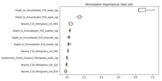

We can see that the weekly lag terms for the two targets are the most important predictors, which is unsurprising. Among the other inputs, the 30-day rolling mean of the volume term and the 120-day rolling mean of the rainfall term are of relatively major importance. Neither of the temperature terms appears in the list of important features at all, perhaps because they had been dropped when we narrowed down the list of features earlier.

Finally, we can calculate the MAE of the predictions. The predictions appear to be reasonably accurate - given that the depth to groundwater terms are in the range of 19 and 35 m, an average absolute error of around 0.3 m is a little over 1%. The RMSE values are also provided below for reference, and are slightly higher than the MAE numbers.

mean_absolute_error(rf_preds_1, test_rf_y, multioutput='raw_values')

mean_squared_error(rf_preds_1, test_rf_y, multioutput='raw_values', squared=False)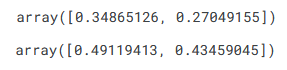

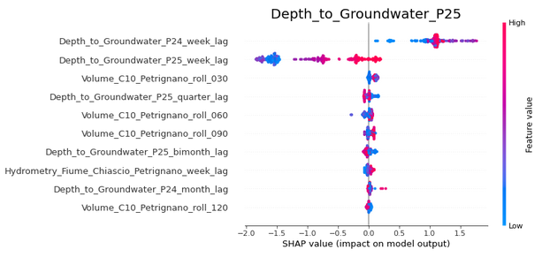
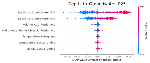
We have looked at the most important features in terms of permutation importance above. Let us now see what the SHAP values calculated using SHAP’s TreeExplainer say. First a look at the summary plot for all the target columns combined:

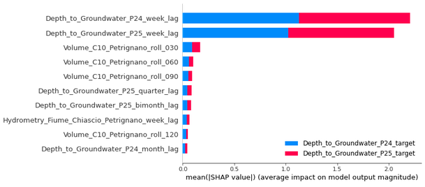
We see that the weekly lag of the two depth to groundwater terms are important predictors for both the target terms, in line with both what the permutation importances showed and our expectations.The 120-day rolling mean of the rainfall is also an important predictor, more for the Depth_to_Groundwater_P24 target than Depth_to_Groundwater_P25 (the blue portion of the bar is longer than the red portion for the Rainfall_Bastia_Umbra_roll_120 term). Three different rolling means of the volume term are of moderate importance, while the weekly lag of the hydrometry term comes much lower down than was the case for the permutation importances. Overall, there is relatively good agreement, but the SHAP plots can provide greater depth of information, as shown below.

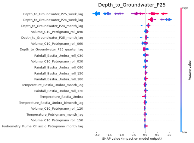
Now let us see what the individual SHAP summary plots show.

i = 0
for target in targets:
    # To ensure the code works if only target variable is present
    if len(targets) == 1:
        shap.summary_plot(shap_values, test_rf_X, show=False)
    else:
        shap.summary_plot(shap_values[i], test_rf_X, show=False)
    plt.title(f'{targets[i]}', fontsize=20)
    plt.show()
    i +=1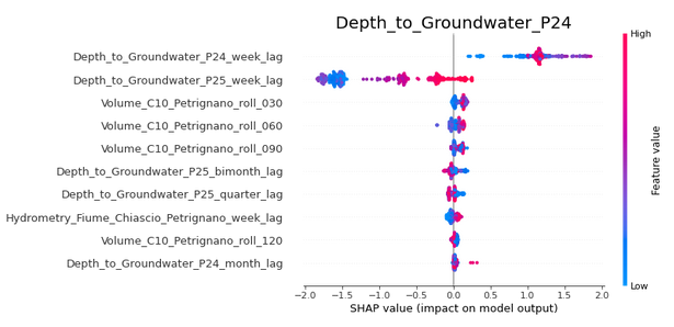

A detailed explanation of how to interpret SHAP summary plots can be found here, but looking at the above, it is clear that they present some interesting insights. Consider the Depth_to_Groundwater_P24 figure. We see that the Depth_to_Groundwater_P24_week_lag term has a positive impact on the model output (except for very low values of the feature), while the Depth_to_Groundwater_P25_week_lag has a negative impact (except for very high values of the feature. Thus, we see that very high values of the Depth_to_Groundwater_P24_week_lag (bright red colour) leads to the model output increasing by around 1.2, while for the Depth_to_Groundwater_P25_week_lag term, very high values affect the model output by -0.2 to +0.1. Very low values of this feature (bright blue) reduce the model output by around 1.5. We also see that the Rainfall_Bastia_Umbra_roll_120 term has a small positive effect, but this effect is a bit inconsistent, as a mixture of blue and red values are seen in the 0.1 to 0.5 region. Finally, all the other terms are centred around 0 with limited spread on either side, indicating that it does not much matter to the model predictions whether these terms have a high or low value - in other words, that they are of low importance in prediction.

The above thus helps us not only see which features are important, but also how they actually impact the model - whether this impact is positive or negative, and whether high values and low values of the feature affect predictions differently. While the above can be discussed in further depth, in the interests of brevity, let us move on to the LGBM model.

LightGBM model

First things first - the LightGBM algorithm does not support multi-output regression, and neither does the competing library XGBoost, for that matter. This hurdle can be tackled in two ways. One is to use sklearns’ MultiOutputRegressor as a wrapper. This works very well indeed, but in our case presents one hitch - SHAP does not support MultiOutputRegressor. This brings us to the second alternative - run LGBM for each target term. This would normally be an inferior alternative, as the interactions between the target terms would not be captured. In this case, for instance, if we run the LGBM for the Depth_to_Groundwater_P24 term, dropping the Depth_to_Groundwater_P25 term, and then the other way round, the effect of the Depth_to_Groundwater_P24 term on the Depth_to_Groundwater_P25 term and vice versa would not be accounted for in the model. Here, though, we are using the lag terms of the targets, which are present during the modelling step, and hence the target variables’ interactions are captured in the model. We will therefore use the LGBMRegressor in a for-loop for each of the target variables. We will stick to the default LightGBM parameters in the interest of time, simplicity, and robustness, but more information about parameter tuning can be found here and here.

The train and test sets are prepared in the same way as for RF, reusing the lag and rolling mean terms we had calculated for using in the RF. As a Gradient Boosting method works sequentially, progressively improving the model to minimise prediction error, a feature selection step as was carried out for the RF is less important - less important features will anyway be dropped as the algorithm finetunes the predictions. In theory, a lower number of features should allow for lower run time, but the feature selection itself is time consuming, and so I did not carry this out for the LGBM model. Therefore, all we now need to do before running the regressor is to drop the Date columns, and create an empty numpy array to hold the model predictions.

regr_lgbm = LGBMRegressor()

train_lgbm_X = rf_X.iloc[:rf_X.loc[rf_X['Date'] == '2019-07-01'].index.item()].reset_index(drop = True)
test_lgbm_X = rf_X.iloc[rf_X.loc[rf_X['Date'] == '2019-07-01'].index.item():].reset_index(drop = True)
train_lgbm_y = rf_y.iloc[:rf_y.loc[rf_X['Date'] == '2019-07-01'].index.item()].reset_index(drop = True)
test_lgbm_y = rf_y.iloc[rf_y.loc[rf_X['Date'] == '2019-07-01'].index.item():].reset_index(drop = True)
# Note that rf_y does not have a Date column, but as it's the same length as rf_X,
# the Date column from that df can be used for the train-test split
train_lgbm_X = train_lgbm_X.drop(['Date'], axis=1)
test_lgbm_X = test_lgbm_X.drop(['Date'], axis=1)

lgbm_preds_1 = np.empty_like(test_lgbm_y)

i = 0
for target in targets:
    m1 = regr_lgbm.fit(train_lgbm_X, train_lgbm_y.iloc[:,i])
    lgbm_preds_1[:,i] = m1.predict(test_lgbm_X)
    explainer2 = shap.TreeExplainer(regr_lgbm)
    shap_values = explainer2.shap_values(test_lgbm_X)
    shap.summary_plot(shap_values, test_lgbm_X, show=False)
    plt.title(f'{targets[i]}', fontsize=20)
    plt.show()
    i +=1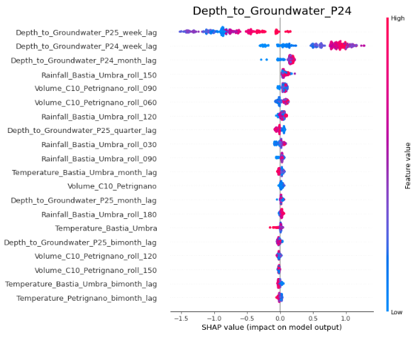

The permutation importances can be calculated for the LGBM similarly to RF, but let us focus on the SHAP summary plots. We see that these are broadly similar to the RF plots, with some differences. In the Depth_to_Groundwater_P24 plot, we see that the impact of the Depth_to_Groundwater_P24 weekly lag term is less pronounced than was the case for RF, with high values increasing model output by less than 1.0. We also see the individual rainfall terms making less of an impact on the model output. These differences are partly a result of the differences in the algorithm, and partly simply due to the greater number of features available to the LGBM regressor, since we did not carry out a feature selection for it. The broad picture, though, remains the same - the weekly lag terms for the depths to groundwater are the most important, the volume and rainfall terms have a part to play, and the hydrometry and temperature terms have a negligible impact on the model output.

Looking at the accuracy of the predictions, we see numbers fairly similar to those obtained for RF.

mean_absolute_error(lgbm_preds_1, test_lgbm_y, multioutput='raw_values')

mean_squared_error(lgbm_preds_1, test_lgbm_y, multioutput='raw_values', squared=False)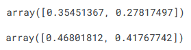

LSTM model

Finally, we come to the LSTM model. The train-test split I did similarly to the RF and LGBM, but the split into the X and y arrays I did as per the code given here. In fact, the LSTM model I used is itself adapted from the ‘LSTM Model With Univariate Input and Vector Output’ section of that page, and hence the explanations given there are applicable here. The only item that needs separate explanation is the scaling step. Scaling is very useful in helping NNs like LSTM make quicker and more accurate predictions, but needs to be carried out post the train-test split to avoid data leakage, which is what has been done below. Sklearn’s MinMaxScaler has been used for scaling.

# Make a copy of the train dataframe
train_lstm = train.copy()
train_lstm = train_lstm.loc[train_lstm.dropna().index[0]:].reset_index(drop = True)
# Create train-test split, then drop Date columns
train_train_lstm = train_lstm.iloc[:train_lstm.loc[train_lstm['Date'] == '2019-07-01'].index.item()]
train_test_lstm = train_lstm.iloc[train_lstm.loc[train_lstm['Date'] == '2019-07-01'].index.item():]
train_train_lstm = train_train_lstm.drop(['Date'], axis=1)
train_test_lstm = train_test_lstm.drop(['Date'], axis=1)
# Create a copy of the train test dataframes and perform scaling on thiese dataframes
# Separate scalers used for the train and test sets to prevent the possibility of data leakage
train_train_lstm2 = train_train_lstm.copy()
train_test_lstm2 = train_test_lstm.copy()
scaler1 = MinMaxScaler()
scaler2 = MinMaxScaler()
train_train_lstm2 = scaler1.fit_transform(train_train_lstm2)
train_test_lstm2 = scaler2.fit_transform(train_test_lstm2)

The function below splits the train and test sets into separate arrays containing the X and y terms, and it is run to obtain the inputs and outputs in the shape required for the LSTM. As mentioned above, the portion below is based on the code here.

# Split a multivariate sequence into samples
def split_sequences(sequences, n_steps):
    X, y = list(), list()
    for i in range(len(sequences)):
        # find the end of this pattern
        end_ix = i + n_steps
        # check if we are beyond the dataset
        if end_ix > len(sequences):
            break
        # gather input and output parts of the pattern
        seq_x, seq_y = sequences[i:end_ix, :-len(target_cols)], sequences[end_ix-1, -len(target_cols):]
        X.append(seq_x)
        y.append(seq_y)
    return array(X), array(y)

# Choose number of time steps used for training. Arbitrary, 7 chosen here.
n_steps = 7

# Convert into input/output
X_train, y_train = split_sequences(train_train_lstm2, n_steps)
print(X_train.shape, y_train.shape)
X_test, y_test = split_sequences(train_test_lstm2, n_steps)
print(X_test.shape, y_test.shape)

# The number of features
n_features = X_train.shape[2]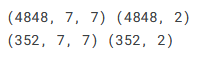

After the preprocessing above, we are ready to define and run the LSTM model. I fit the model for 200 epochs, as I found this to give good results while taking a reasonable amount of time. If necessary the ideal number of epochs can be figured out as shown here, but let’s leave that for now.

# Define model
model = Sequential()
model.add(LSTM(100, activation='relu', return_sequences=True, input_shape=(n_steps, n_features)))
model.add(LSTM(100, activation='relu'))
model.add(Dense(len(target_cols)))
model.compile(optimizer='adam', loss='mse')

# Fit model
model.fit(X_train, y_train, epochs=200, verbose=0)

# Demonstrate prediction
yhat = model.predict(X_test, verbose=0)

# Change X test array dimensions and concatenate with y test and y prediction arrays
X_test_new = X_test[:,0,:]
test_new = np.concatenate((X_test_new, y_test), axis=1)
test_new2 = np.concatenate((X_test_new, yhat), axis=1)

# Scale back the test arrays
test_new = scaler2.inverse_transform(test_new)
test_new2 = scaler2.inverse_transform(test_new2)

# Create target and prediction arrays containing only the target terms, to compare the predictions
y_targets = test_new[:, -len(target_cols):]
lstm_preds_1 = test_new2[:, -len(target_cols):]

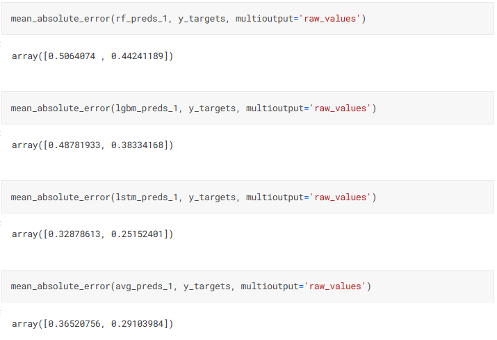
Looking at the MAE values, we see that the LSTM model is more accurate for this waterbody than the RF and LGBM models.

mean_absolute_error(lstm_preds_1, y_targets, multioutput='raw_values')

mean_squared_error(lstm_preds_1, y_targets, multioutput='raw_values', squared=False)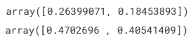

The SHAP analysis of the LSTM cannot be done by the TreeExplainer like for the tree-based models, and the DeepExplainer available for NNs gives errors like this for LSTMs, and so I used the GradientExplainer instead. The difference in the SHAP summary plots for LSTM as compared to the earlier plots is obvious - the Depth_to_Groundwater terms are used directly in the LSTM for predictions, and hence high values of these variables give high values for the model output, and the other way around. This shows that the influence of a feature on the prediction depends not only on the variable but also on the type of model used.

explainer = shap.GradientExplainer(model, X_train)
shap_values1 = explainer.shap_values(X_test)
Xtests = np.hsplit(X_test, n_steps)
i = 0
for target in targets:
    shaps = np.hsplit(shap_values1[i], n_steps)
    shap.summary_plot(np.squeeze(shaps[n_steps-1]), np.squeeze(Xtests[n_steps-1])
                      ,feature_names = train_test_lstm.columns.tolist(), show=False)
    plt.title(f'{targets[i]}', fontsize=20)
    plt.show()
    i +=1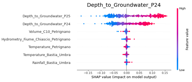

Ensembling

We have seen that all the models gave quite good results on the Petrignano dataset. Let us now see how an ensemble of these models fares. First we need to reshape the different model prediction arrays to make these all the same shape. Then we take an average of the predicted values, and find the MAE.

rf_preds_1 = np.delete(rf_preds_1, np.s_[0:n_steps-1], axis=0)
lgbm_preds_1 = np.delete(lgbm_preds_1, np.s_[0:n_steps-1], axis=0)
lstm_preds_1 = lstm_preds_1.reshape(rf_preds_1.shape)
avg_preds_1 = (rf_preds_1 + lgbm_preds_1 + lstm_preds_1)/3

mean_absolute_error(avg_preds_1, y_targets, multioutput='raw_values')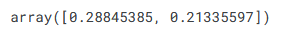

We see that the ensemble produces results that are slightly inferior to the best model here, the LSTM. Two comments can be made on this. Firstly, we have used a simple average of the predictions here. Using a meta model to stack these predictions will almost certainly result in more accurate predictions. The downside is that stacked models are significantly slower and more computationally expensive. As I had already developed some very elaborate models that took a fair amount of time to run, I decided that a simple average would suffice here instead of adding further complications. The other point is that the benefit of ensembling will be more clearly brought out when I touch upon some of the other water bodies next time.

Forecast period of 30 days

I reran all the code for a forecast period of 30 days - everything remaining identical, except putting days_ahead = 30. The model ran smoothly and automatically, producing predictions that are slightly less accurate, understandable given that the prediction period is further away:

Conclusion

That pretty much covers everything I had to say about Aquifer Petrignano. The next time, we will take a brief look at some of the interesting points in the modelling of the other water bodies to wind up this series. So long!