Modelling water bodies - 4 | Agneev’s DS/ML lab book

Categories:

Data Science Machine Learning Python Time series Tabular

Tags:

Environment, Water, Kaggle, Competition, Matplotlib

Welcome to the last post in the water body modelling series! The last time we saw the modelling of the Aquifer Petrignano using a Random Forest, a LightGBM and an LSTM model, for two different forecast periods. We also saw how to analyse their feature importance via permutation importance and SHAP. It would be redundant (and boring!) to look at all that again for each of the nine water bodies, and so in this post I will just highlight some of the interesting points that arose for the other water bodies. As I say each time, you can find all the code here.

Aquifer Auser

As per the competition page,

This waterbody consists of two subsystems, called NORTH and SOUTH, where the former partly influences the behavior of the latter. Indeed, the north subsystem is a water table (or unconfined) aquifer while the south subsystem is an artesian (or confined) groundwater.

The levels of the NORTH sector are represented by the values of the SAL, PAG, CoS and DIEC wells, while the levels of the SOUTH sector by the LT2 well.

So what is interesting about the modelling of this particular water body? Let us examine the hydrometry chart:

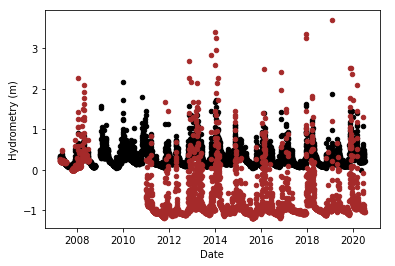
Here we see one aspect that differs from the Petrignano dataset. It appears that the following a long break, the Piaggione hydrometry level has been moved down, in relation to both its pre-break levels and Monte_S_Quirico (the black series) levels. This most likely indicates an error. It would probably be sensible to move it up by the difference in the minima of the pre-and post-break values. The other option would be to move the first part down, but since all the other hydrometry terms lie in the positive region, I went with the moving up option. In any case, it’s the inconsistency in the before and after value that is important; the models will be able to handle the absolute values.

The post-break appears to start around early 2011, so first let’s verify this. Let’s get the row number:

train.loc[train['Date'] == '2011-01-01']

	Date	Rainfall_Gallicano	Rainfall_Pontetetto	Rainfall_Monte_Serra	Rainfall_Orentano	Rainfall_Borgo_a_Mozzano	Rainfall_Piaggione	Rainfall_Calavorno	Rainfall_Croce_Arcana	Rainfall_Tereglio_Coreglia_Antelminelli	Temperature_Monte_Serra	Temperature_Ponte_a_Moriano	Temperature_Lucca_Orto_Botanico	Volume_POL	Volume_CC1	Volume_CC2	Volume_CSA	Volume_CSAL	Hydrometry_Monte_S_Quirico	Hydrometry_Piaggione
1363	2011-01-01	0.0	0.0	0.0	0.0	0.0	0.0	0.0	0.0	0.2	3.6	6.4	4.9	-10080.64516	-16485.10963	-13875.84	0.0	0.0	0.5	-0.33

‘Hydrometry_Piaggione’ is the last column in the table, so:

train.iloc[1355:1370,-1]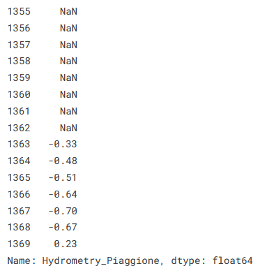

We can see that there is indeed a bunch of NaNs here, so let us now move up the 2nd part by the difference between the minima of the 1st and 2nd parts, and then re-plot.

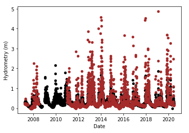
This looks much better, and after imputation we get:

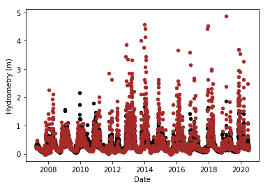
This looks just fine.

Another important aspect is the ensembling. Let us look at the results of the three individual models and the ensemble:

Here we see the benefit of using a range of models. The LSTM, which had given the best predictions for Petrignano, gives the worst results for Auser, but ensembling enables us to mitigate the inaccuracy, even if the final predictions are still worse than those given by the tree-based methods.

Aquifer Doganella

The wells field Doganella is fed by two underground aquifers not fed by rivers or lakes but fed by meteoric infiltration. The upper aquifer is a water table with a thickness of about 30m. The lower aquifer is a semi-confined artesian aquifer with a thickness of 50m and is located inside lavas and tufa products. These aquifers are accessed through wells called Well 1, …, Well 9. Approximately 80% of the drainage volumes come from the artesian aquifer. The aquifer levels are influenced by the following parameters: rainfall, humidity, subsoil, temperatures and drainage volumes.

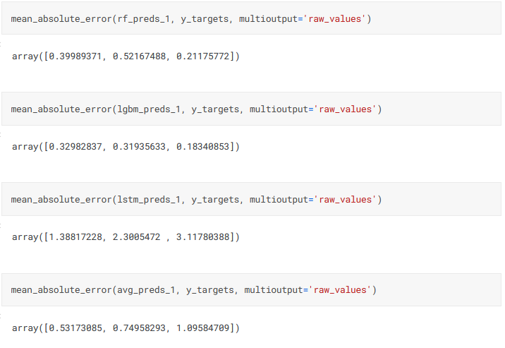
The benefits of ensembling are demonstrated even better in this dataset. First let us see the results for each term, using code like:

mean_absolute_error(rf_preds_1, y_targets, multioutput='raw_values')

mean_absolute_error(lgbm_preds_1, y_targets, multioutput='raw_values')

mean_absolute_error(lstm_preds_1, y_targets, multioutput='raw_values')

mean_absolute_error(avg_preds_1, y_targets, multioutput='raw_values')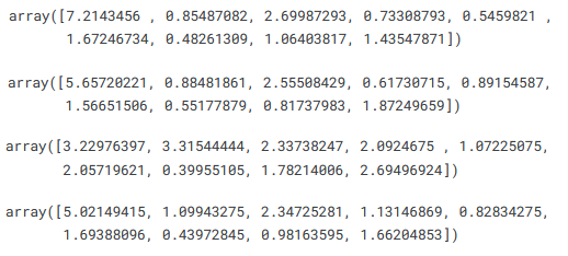

We see that each model gives the best prediction for 3 targets out of 9, and the ensemble is able to give more accurate predictions on the whole than is the case for any individual model. This can be crosschecked by looking at the uniform average errors below.

mean_absolute_error(rf_preds_1, y_targets, multioutput='uniform_average')

mean_absolute_error(lgbm_preds_1, y_targets, multioutput='uniform_average')

mean_absolute_error(lstm_preds_1, y_targets, multioutput='uniform_average')

mean_absolute_error(avg_preds_1, y_targets, multioutput='uniform_average')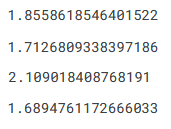

Aquifer Luco

The Luco wells field is fed by an underground aquifer. This aquifer not fed by rivers or lakes but by meteoric infiltration at the extremes of the impermeable sedimentary layers. Such aquifer is accessed through wells called Well 1, Well 3 and Well 4 and is influenced by the following parameters: rainfall, depth to groundwater, temperature and drainage volumes.

The main thing I want to show about aquifer Luco is the poor quality of some of the data. Have a look at the ‘Depth to Groundwater’ data:

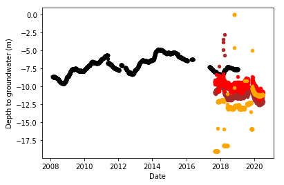
Imputing with MissForest gives:

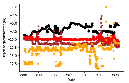
This looks fairly reasonable, but is it? The large chunks of missing data means there is no way to tell. Imputing over such a large span of time is unwise, and should be avoided unless there is no alternative. In either case, the lack of data for these terms made forecasting for this water body difficult, with the best error obtained (0.466 for the ensemble) amounting to well over 5% error.

Water spring Amiata

The Amiata waterbody is composed of a volcanic aquifer not fed by rivers or lakes but fed by meteoric infiltration. This aquifer is accessed through Ermicciolo, Arbure, Bugnano and Galleria Alta water springs. The levels and volumes of the four sources are influenced by the parameters: rainfall, depth to groundwater, hydrometry, temperatures and drainage volumes.

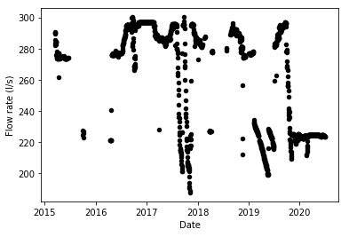
Modelling the water springs follows essentially the same format as the aquifers, except that the type of input variables is a little different (flow rate in place of volume and hydrometry). Let us just look at the flow rate term.

The flow rates refer to, as expected, the water flow rate of the spring. Looking at the above graphs, two things stand out - the 0s are likely to be errors, and since the data are in the form of a continuous series, rolling means are an appropriate interpolation method. Imputation was therefore simply done by:

if len(flows)>0:
    i = 0
    while i<len(flows):
        train[f'{flows[i]}'].replace(0, np.nan, inplace=True)
        i += 1

# 0s in flows are errors, so replace them with Nans

There isn’t much else that is different here, so let’s move on to the next water body.

Water spring Lupa

This water spring is located in the Rosciano Valley, on the left side of the Nera river. The waters emerge at an altitude of about 375 meters above sea level through a long draining tunnel that crosses, in its final section, lithotypes and essentially calcareous rocks. It provides drinking water to the city of Terni and the towns around it.

A cursory look at this dataset is enough to show that it is different:

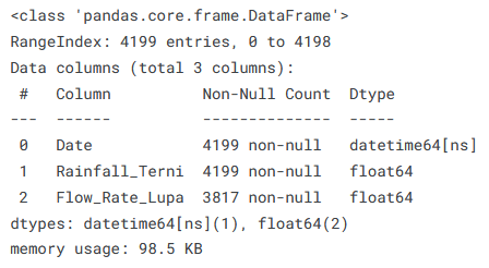
That’s right, a single ‘X’ or exogenous term - ‘Rainfall_Terni’, and a single ‘Y’ or target term - ‘Flow_Rate_Lupa’. As if that wasn’t enough, look at the rainfall term:

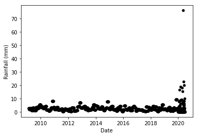
The values of Rainfall_Terni are given as monthly averages for the period from 2009 to 2019, but as daily data in 2020. This means that the test data is considerably different from the training data, further compounded by one day in 2020 receiving 76 mm of rainfall, by far the highest value. To be able to model this dataset, I had to replace the 2020 daily rainfall data by the monthly average. First I located the row at which 2020 started:

rain_df.iloc[3965:3970]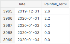

Then I made a new dataframe for the 2020 rainfall:

rains_2020 = rain_df.iloc[3966:]

Replace by the monthly average:

rains_2020['Rainfall_Terni'] = rains_2020.groupby(pd.Grouper(key='Date', freq='M')).transform('mean')

Insert the newly averaged terms back into the original dataframes and plot the new data:

rain_df.Rainfall_Terni.iloc[3966:] = rains_2020.Rainfall_Terni.iloc[:]

train.Rainfall_Terni.iloc[3966:] = rain_df.Rainfall_Terni.iloc[3966:]

if len(rains)>0:
    i = 0
    while i<len(rains):
        if i == 0:
            ax1 = rain_df.plot.scatter(x = 'Date', y = f'{rains[i]}', color=colours[i])
        else:
            axes = rain_df.plot.scatter(x = 'Date', y = f'{rains[i]}', color=colours[i], ax = ax1)
        y_axis = ax1.yaxis
        y_axis.set_label_text('Rainfall (mm)')
        i += 1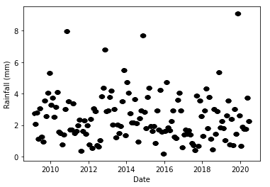

This now looks quite reasonable…

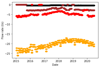
What about the other term, the one we are supposed to predict for?

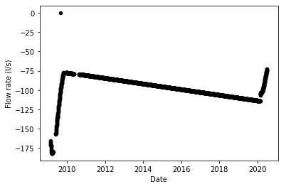
I think you can see why this waterbody was the cause of a lot of anguished comments on the competition forums…

Water spring Madonna di Canneto

The Madonna di Canneto spring is situated at an altitude of 1010m above sea level in the Canneto valley. It does not consist of an aquifer and its source is supplied by the water catchment area of the river Melfa.

Speaking of the data causing anguish, I will just show a couple of graphs for this water spring and leave it at that:

That’s not too bad, but this…

I am actually quite fond of this graph, as it is something I like to present as an ‘Exhibit A’ of bad data…

River Arno

Arno is the second largest river in peninsular Italy and the main waterway in Tuscany and it has a relatively torrential regime, due to the nature of the surrounding soils (marl and impermeable clays). Arno results to be the main source of water supply of the metropolitan area of Florence-Prato-Pistoia. The availability of water for this waterbody is evaluated by checking the hydrometric level of the river at the section of Nave di Rosano.

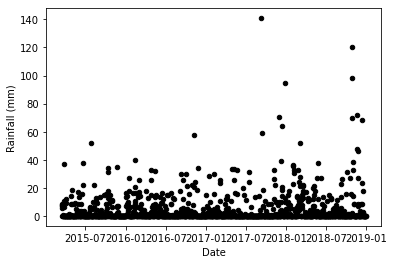
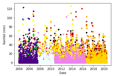
This is the only river in the competition, and is actually entirely unremarkable, so much so that I did not make a single specific comment on it in my competition submission notebook. Perhaps the most noteworthy thing would be the rainfall graph below, showing the different rainfall terms having different years of missing data…

Lake Bilancino

Bilancino lake is an artificial lake located in the municipality of Barberino di Mugello (about 50 km from Florence). It is used to refill the Arno river during the summer months. Indeed, during the winter months, the lake is filled up and then, during the summer months, the water of the lake is poured into the Arno river.

This is the final water body in the competition dataset, and the only lake. Its modelling is largely similar to the rest, except that it has a ‘Lake_Level’ term, which is one of the targets, and the ‘Flow_Rate’, the other target, differs in meaning from the water spring flow rates.

First, the lake level looks like this:

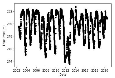
It exhibits a distinct degree of seasonality, and hence I used seasonal interpolation for data imputation, similarly to temperature.

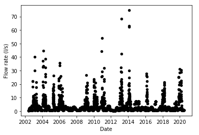
The above shows the flow rate, which, as I said, is different from what it meant in the water springs. Here it refers to the flow rate at the water withdrawal station, and hence is comparable with the volume term in the aquifers. In other words, it can be 0, and therefore imputation can only be done by filling with 0s.

Conclusion

And that’s it! It’s been a long trip through the different water bodies and the quirks associated with their modelling, but worthwhile, I hope. One of the frustrations of this competition was that the winning submissions were never released, preventing people from learning from these. I quite liked my own submission, except that it was very long (like these posts…), and in hindsight, I would have skipped some of the figures for the latter waterbodies to reduce the length and the monotony. Oh well, I at least hope the organisers got what they wanted from the competition. I will leave you with my final words from my competition entry, which I think still sum up my feelings well:

This notebook presents models for forecasting the target terms for four different types of waterbodies, with the ensembling of random forest, gradient boosting and neural networks providing accurate and reliable predictions for any desired time period. Overall, this competition was a great learning experience, and I would like to thank the organisers for this. One issue is regarding the quality of data, which for some waterbodies, especially water springs Lupa and Madonna di Canneto, were scarce and of poor quality, severely hampering the quality of the model predictions. Ultimately, no amount of sophistication in data imputation and modelling can compensate for a lack of appropriate and sufficient data, and therefore addressing this should be the first step taken towards being able to better forecast water availability. Overall, though, this analytics competition was a great initiative, and I hope that the outcome of the competition will not only help Acea better manage its waterbodies, but will also spur a general interest in applying such techniques to water management.